

Reinforced concrete (RC) core walls are a common structural system in the construction of tall buildings, valued for their rapid construction timeline and the architectural flexibility they provide around the building core. Economically, it is recognized that during a design-based earthquake (DBE) or maximum considered earthquake (MCE), some degree of plastic deformation within the core wall system is inevitable. Consequently, building codes specify the use of reduced lateral forces for design, explicitly allowing for the development of plasticity in certain structural elements during major seismic events. For cantilever walls, the intended location for this inelastic flexural deformation is at the base, an area designated as the plastic hinge region. Multiple studies recommend concentrating a single plastic hinge at the wall’s base, with the condition that its rotation is carefully controlled, while the upper sections of the wall are expected to remain elastic [1-4]. This concentration of plasticity at the base is the traditional and preferred failure mechanism for cantilever RC walls [5].
Within these plastic hinge regions, special reinforcing bar detailing is essential to withstand the large deformation demands of strong earthquakes. The walls must demonstrate the ability to develop a ductile flexural plastic hinge at their base, doing so without significant shear distress or other failure modes that lead to a rapid loss of strength under cyclic inelastic loading [6].
Research has shown that the dynamic response of tall cantilevered walls is significantly influenced by higher-mode effects. Numerical and experimental studies confirm that strong ground motions can generate larger-than-anticipated moment demands at the mid-height and increased shear demands at the base of these systems [7-13].
Furthermore, studies indicate that while a base plastic hinge primarily reduces the contribution of the first vibration mode, higher modes are not dampened to the same extent. This leads to a relative increase in the influence of higher modes on the overall structural response. As a result, the Response Spectrum Analysis (RSA) procedure, which is designed for linear systems and recommended by many codes, is considered inadequate for designing nonlinear cantilever RC walls with a localized nonlinear base zone [4]. Experimental evidence also points to the potential for a plastic hinge to form above the base of an RC wall [9]. For instance, tests on a seven-storey wall noted higher-mode effects, though these were not pronounced enough to push plasticity above the base [14]. However, historical data does show instances of plastic hinges forming at intermediate heights. The likelihood of this occurring increases with building height and when reinforcement is curtailed along the wall’s height [11,15]. When significant energy dissipation occurs in the upper stories of a reinforced concrete (RC) wall, the resulting damage can be both widespread and difficult—if not prohibitively expensive—to repair. To address this issue and better control how plasticity and energy dissipation are distributed throughout tall core-wall systems, this study proposes a combined structural solution: integrating buckling-restrained braced frames (BRBFs) into the design. This hybrid approach offers a promising path toward mitigating upper-level damage while enhancing the overall energy absorption strategy of the system.
The buckling-restrained brace (BRB) is a relatively recent development of energy-dissipating elements suitable for tall buildings. Concentrically braced frames with these elements, BRBFs have received considerable attention from researchers and practitioners for their seismic performance. The most important advantage of BRBs over regular steel braces relates to their ability to prevent buckling in compression. Their design was arranged to yield and dissipate seismic energy effectively in both tension and compression [15-18]. Regular braces buckle under compression and, therefore are not able to utilize their compressive strength effectively, resulting in severely deteriorated hysteretic behavior during strong ground motions. The basic concept of a BRB is a steel core enclosed in a confining system so that it can yield in compression without buckling. Confinement is commonly provided with concrete-filled steel tubes and several experimental tests have demonstrated that BRBs with this configuration have significant energy dissipation and ductility [19,20]. Tremblay et al. [21] carried out one of the first series of tests on BRBs for a seismic retrofitting project in Canada.
Subsequent experimental and numerical studies on large-scale BRBFs with different configurations have shed more light on their seismic behavior [22-27]. These studies confirmed the ductility and energy dissipation capabilities of BRBs, which perform well under design-level earthquake demands and beyond. However, a potential drawback came to light: a tendency for significant residual drift [28]. Several studies have quantified the range of story drift and deformation demands expected in BRBFs [27,29-32]. Compared to conventional Concentrically Braced Frames, BRBFs have lower initial and post-yield stiffness, and hence are more susceptible to soft-story mechanisms. Desirable is a design outcome featuring multiple stories with significant yielding. In BRBFs, drift tends to concentrate in a single story because yielding of the BRBs in that story causes its stiffness to drop steeply. This concentration is problematic in that it can lead to global instability due to P-Delta effects, and result in large permanent residual drifts. A promising strategy for mitigating this problem is combining BRBFs with an RC wall.
Forward directivity, or pulse-like, ground motions can impose exceptionally large deformation and strength demands on structures, often resulting in more severe damage compared to ordinary far-fault (FF) motions [33-39]. This pulse effect is a major characteristic of near-fault (NF) ground motions and a primary cause of extensive structural damage. The influence of forward directivity diminishes with distance from the fault; beyond 10 to 15 km from the rupture, such pulse-like motions are unlikely to occur [40].
The characteristics of a near-fault motion are influenced by the shaking intensity, the geometry of the fault, and the orientation of the seismic waves [41]. A pulse is most commonly observed in the velocity time-history, making the velocity pulse a more widely used indicator of damage potential in earthquake engineering than pulses in acceleration or displacement records. The maximum displacement during these pulse-like motions is also closely linked to their potential for causing collapse and severe damage [42].
Since the 1950s, the concept of energy has been a compelling topic for researchers seeking to improve seismic design methodologies [43-44]. An energy-based approach offers a foundation for estimating expected seismic demands and can indirectly gauge the destructive potential of an earthquake. Several methodologies that account for input and dissipated energy have been proposed by researchers [37,45,46].
Measurements of the energy input into structures from various earthquakes have been conducted [47-48]. These investigations have shown that hysteretic energy input is a useful parameter for explaining structural damage and performance demands.
The analysis of energy in tall core-wall systems integrated with BRBs is a novel and relevant area of study. Energy demand is regarded as a reliable metric for predicting seismic hazard. Many researchers have employed this approach by evaluating the total input energy [49]. Near-fault earthquakes are particularly destructive due to the instantaneous energy demand caused by extreme pulse effects, which force structures to undergo large nonlinear deformations in just a few cycles. In these events, damage is dominated by peak demands rather than the cumulative effects of low-cycle fatigue. Records with strong acceleration pulses can cause a sudden, large rise in energy input early in the response, which can be substantially greater than the total energy accumulated by the end of the shaking [50].
The unique properties of forward directivity records can force a structure to dissipate the earthquake’s input energy through a few large plastic cycles. Examining how energy demand fluctuates during an earthquake, alongside structural properties, can lead to a more precise understanding of seismic demands [50,51].
Earthquake input energy serves as an effective intensity measure for near-fault ground motions [52]. This parameter is advantageous because it accounts for both ground motion characteristics (like duration and frequency content) and structural properties (such as ductility, damping, and hysteretic behavior). Consequently, it provides a more comprehensive measure of earthquake intensity compared to other common parameters like Peak Ground Acceleration (PGA) or Spectral Intensity [53].
The energy demands for tall RC core-walls combined with BRBF subjected to the NF and FF earthquake records have not been investigated yet. BRBF can contribute in energy dissipation and reduce the damage of the RC core-walls over the height and cause the less inelastic energy demand in the RC core wall. In the present research, BRBF has been added to the RC core- wall and a new combined core system has been developed. Fiber element model has been applied for RC wall model as well as appropriate nonlinear elements have been used to make nonlinear models.
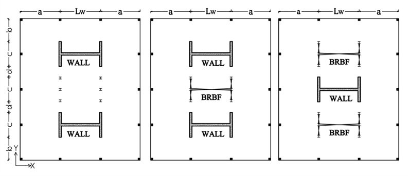
This research focused on 40-story structures, with each story having a standard height of 3.5 meters. For the design phase, three-dimensional linear elastic models of the structural systems were created using the ETABS software [54]. The study examined three distinct core configurations:
The 2BRB+1RC model, featuring two I-shaped Buckling-Restrained Braced Frames (BRBFs) and one I-shaped Reinforced Concrete (RC) wall in its plan.
The 1BRB+2RC model, composed of one I-shaped BRBF and two I-shaped RC walls.
The 2RC model, which served as a benchmark and contained only two I-shaped RC walls, a configuration deemed sufficient to meet code requirements without additional elements. The layout of these core systems is provided in Figure 1.
The floors were constructed from RC slabs. Within the software, the shear walls were modeled using shell-type plate elements. These elements employ a triangular or quadrilateral formulation that integrates membrane and plate-bending behaviors, with six degrees of freedom at each node. The distributed dead and live loads on the floors were specified as 7 \(\frac{\mathrm{KN}}{\mathrm{m}^2}\) and 2 \(\frac{\mathrm{KN}}{\mathrm{m}^2}\), respectively, and the corresponding tributary loads carried by the core systems were applied. A rigid diaphragm constraint was used, with the mass of each story assigned to its center of mass. The foundation connections for the walls were modeled as fixed, while those for the columns and the beam-to-column connections in the BRBFs were modeled as pinned. The core system was designed to resist all lateral seismic loads, while both the peripheral columns and the core shared the vertical dead and live loads. Given the assumption that the core alone carries the lateral load, the gravity-only elements (floors and peripheral columns) were omitted from the numerical model used for design, as their influence on lateral stiffness has been shown to be insignificant in previous studies [55]. However, the gravity load supported by the core itself was included in the model.
In accordance with ASCE 7 [56], the design employed response modification factors (R) of 5 for special RC walls and 8 for BRBFs. For the combined systems, the more conservative value of R=5 was applied, as prescribed by the code when different structural systems interact. The base shear force derived from Response Spectrum Analysis (RSA) was adjusted such that it was not less than 90% of the base shear from the equivalent lateral force procedure, effectively defining an effective response modification factor for the RSA process.
The systems were designed following the standards of ASCE-7 and ACI318-11 [56-57]. The concrete in the RC walls had a nominal compressive strength of 45 MPa, and the steel reinforcement had a nominal yield strength of 400 MPa. To account for the effect of cracking on the lateral stiffness of the RC walls, their flexural stiffness was reduced by applying a factor of 0.5 to the moment of inertia of the cross-section, consistent with the recommendations of ACI 318-11 (Sections 8.8 and 10.10).
The BRBFs were designed according to standard prescriptive code criteria. The axial load capacity of the buckling-restrained braces was determined as \(\mathrm{\phi}A_sF_y\), where \(\mathrm{\phi}\) = 0.9, \(F_y\) = 250 MPa, and \(A_s\) is the cross-sectional area of the brace element in the elastic model [58]. As per AISC’s Seismic Provisions [59], columns in BRB frames were designed for the combined axial and moment demands from code-level forces, as well as for the axial load resulting from the expected vertical components of all BRBs attached to the column. The maximum expected compression force in a brace was calculated as \(R_y \omega \beta A_s F_y\), where the material over-strength factor \(R_y\) = 1.1, the strain-hardening factor \(\omega\) = 1.25, and the compression overstrength factor \(\beta\) = 1.1 [60].
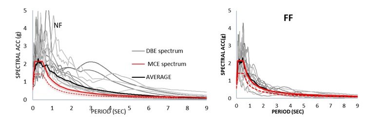
The structural analysis and design for this study were conducted exclusively for loading in the X direction, a methodological approach also adopted in prior research [11]. Response Spectrum Analysis (RSA) was employed for the structural evaluation, from which the natural periods, mode shapes, and modal mass participation factors were determined. The results indicated that the first four translational vibration modes in the X direction collectively account for over 90% of the participating modal mass. The design demands were calculated using a 5% damped Design Basis Earthquake (DBE) response spectrum during the RSA procedure, as illustrated in Figure 2.
A consistent layout of vertical reinforcement was applied throughout the RC wall sections. The vertical reinforcement ratio was held constant over every 10% segment of the building’s height. The computed values for this ratio are provided in Table 1.
| 2RC | 1BRB+2RC | 2BRB+1RC | |||||
|---|---|---|---|---|---|---|---|
| No. of stories | \(\rho\) | \(\rho\) | BRB core cross- section area cm2 |
Column section profile |
\(\rho\) | BRB core cross- section area cm2 |
Column section profile |
| 1-4 | 1 | 1.03 | 7 | W30X326 | 1.58 | 17 | W36X652 |
| 5-8 | 0.68 | 0.75 | 11 | W27X307 | 1.11 | 16 | W40X593 |
| 9-12 | 0.48 | 0.47 | 11 | W27X281 | 0.8 | 32 | W40X593 |
| 13-16 | 0.39 | 0.37 | 16 | W27X281 | 0.68 | 42 | W40X431 |
| 17-20 | 0.4 | 0.37 | 25 | W27X235 | 0.64 | 42 | W40X362 |
| 21-24 | 0.4 | 0.39 | 25 | W21X166 | 0.62 | 42 | W40X362 |
| 25-28 | 0.38 | 0.38 | 25 | W21X132 | 0.57 | 42 | W36X232 |
| 29-32 | 0.32 | 0.32 | 25 | W16X100 | 0.48 | 42 | W36X210 |
| 33-36 | 0.25 | 0.25 | 17 | W14X53 | 0.3 | 42 | W27X114 |
| 37-40 | 0.25 | 0.25 | 16 | W14X34 | 0.25 | 32 | W27X102 |
| ITEM | 2RC | 1BRB+2RC | 2BRB+1RC | |
|---|---|---|---|---|
| H t (m) | 140 | 140 | 140 | |
| Seismic Weight, W (Tonf) | 41290 | 40380 | 38850 | |
| Lw (m) | 12 | 12 | 12 | |
| a (m) | 10 | 10 | 10 | |
| b (m) | 6.5 | 6.5 | 6.5 | |
| c (wall flange) (m) | 7 | 7 | 7 | |
| d (m) | 3 | 3 | 3 | |
| Wall thickness (m) | 0.7 | 0.65 | 1.10 | |
| P/(Ag.fc) | 0.12 | 0.124 | 0.091 | |
| boundary zone height (No. of stories ) | 1-28 | 1-29 | 1-26 | |
| Design base shear, Vrsa, (Tonf) | 2515 | 2462 | 2358 | |
| Effective response modification factor (Reff) | 3.71 | 3.66 | 3.56 | |
| Period of free vibration (s) | T1 | 5.15 | 5.15 | 5 |
| T2 | 0.877 | 0.896 | 0.929 | |
| T3 | 0.354 | 0.35 | 0.376 | |
| Modal P.M.R | Mode 1 | 0.63 | 0.63 | 0.63 |
| Mode 2 | 0.20 | 0.20 | 0.20 | |
| Mode 3 | 0.07 | 0.07 | 0.07 | |
| Mode 4 | 0.035 | 0.035 | 0.034 | |
| Lateral Stiffness (Tonf/m) | RC walls | 2406 | 2144 | 1884 |
| BRBFs | – | 76 | 331 | |
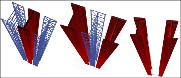
The boundary elements at the base of the RC walls extended upward for 65%, 72.5%, and 70% of the total wall height in the 2BRB+1RC, 1BRB+2RC, and 2RC models, respectively. A minimum longitudinal reinforcement ratio of 0.25% was maintained in accordance with code requirements [57]. The building’s aspect ratio, defined as the total height divided by its width in the X direction, was approximately 4.4. Further details on the designed system are presented in Table 2. The thickness of the walls remained uniform over the entire height of the structure. The elastic finite element model created in ETABS software is depicted in Figure 3.
To accurately capture the realistic seismic performance of the core systems under investigation, nonlinear models were constructed in Perform-3D software [61]. The modeling approach employed fiber elements for the reinforced concrete (RC) walls and specific BRB elements for the braces. Steel columns were represented using concentric axial-moment hinges, while beams were modeled as elastic members. A rigid diaphragm constraint was applied to the floors, with the mass property assigned to the center of mass for each story.
The fiber element method’s capability to accurately simulate the response of RC shear walls is well-established in research [62]. Studies comparing fiber model predictions against experimental data from large-scale slender concrete shear wall specimens under cyclic loading have shown strong correlation. This method is extensively used to predict RC wall behavior under both static and dynamic loads and offers distinct advantages over lumped-plasticity beam-column models. For instance, fiber element modeling can effectively predict the migration of the neutral axis that occurs under lateral loading [63].
To validate the accuracy of the modeling approach for shear wall elements, results from an experimental program by Thomsen and Wallace [64] on a slender RC shear wall under cyclic lateral loading were used [64]. The test specimen, a rectangular shear wall designated RW2, is shown in Figure 4. This wall was capacity-designed to form a flexural hinge at its base. For the simulation, it was modeled using five nonlinear shear wall elements, as depicted in Figure 5. To account for the concentration of inelastic strain, the element length at the base was set equal to the assumed plastic hinge length of \(0.5L_w\), where \(L_w\) is the length of the core wall. The global lateral force versus top displacement response has been shown to be largely insensitive to mesh size and the number of material fibers [62]. Furthermore, according to Powell [2], a single element per story height is generally adequate for simulating shear wall behavior outside the hinge region [62].
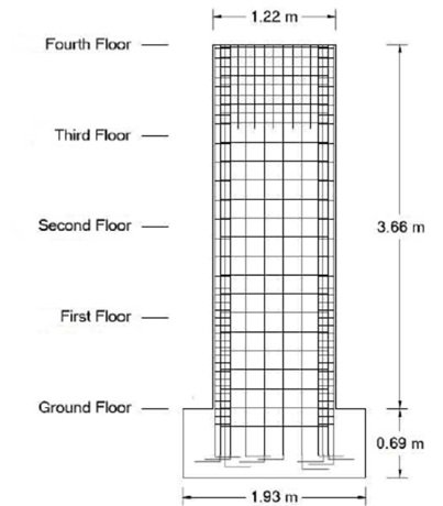
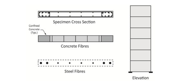
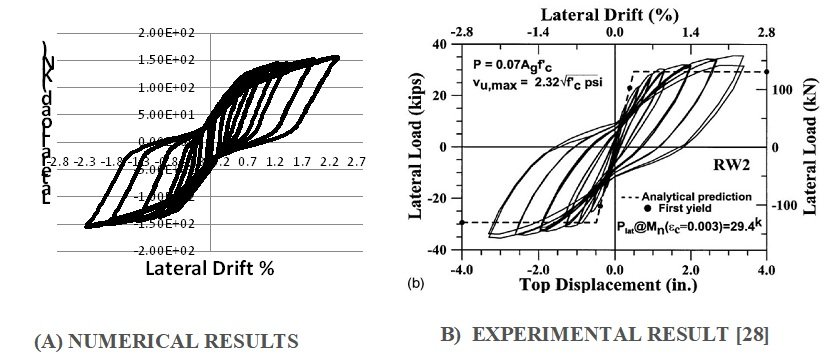
The shear wall elements were designed to exhibit inelastic behavior in bending and/or shear along their longitudinal direction. The “shear wall, inelastic section” component within the software was used to define the wall section properties. In the nonlinear zones of the core wall models, each shear wall element was discretized into eight vertical nonlinear concrete fibers and eight vertical nonlinear steel fibers. Out-of-plane bending was considered secondary and was modeled with linear elastic assumptions [66]. The model replicated the test conditions, wherein a constant axial load of approximately \(0.07A_gf_c'\) (where \(A_g\) is the wall cross-sectional area and \(f_c'\) is the concrete compressive strength from the test) was applied. Cyclic lateral displacements were then imposed at the top of the wall. A comparison between the numerical and experimental hysteresis results is presented in Figure 6, with the horizontal axis representing the lateral drift at the roof of the specimen.
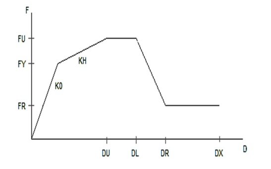
The BRB component in Perform-3D is modeled as an axial element that resists only axial forces and offers no torsional or bending resistance. This component is composed of two segments in series: a linear, non-yielding portion and a nonlinear, yielding portion. The length assigned to the restrained, nonlinear segment is typically 70% of the total brace length between nodes, with the remaining 30% designated as the linear, non-yielding part. This linear portion generally comprises the transition and end segments, as illustrated in Figure 7.

To ensure that inelastic deformation is confined to the central core, the cross-sectional areas of the transition segment (\(A_t\)) and end segment (\(A_e\)) are designed to be larger than that of the yielding core. For the BRB elements in this study, these areas were specified as 1.6 and 2.2 times the core cross-sectional area, respectively. The lengths of the transition and end segments were defined as 0.06 and 0.24 of the total brace length [67].
The cross-sectional area of the yielding core (\(A_c\)) for the BRB element was determined using the following equation [68]:
\[\label{eq1} \frac{L_c}{A_c}\mathrm{=}\frac{L_w}{A_{eq}}\mathrm{-}\frac{L_e}{A_e}\mathrm{-}\mathrm{\ }\frac{L_t}{A_t},\tag{1}\] where Lc, Lt, Le and Lw represent the lengths of the yielding core, transition segment, end segment and the whole bracing, respectively; Also, Aeq is the cross section area of the equivalent bar calculated from the linear design procedure. [69].
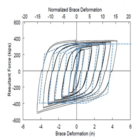
The verification of the BRB elements was calibrated by a test result [2]. Load-deformation graph of BRBs has been illustrated in Figure 8. The force-displacement hysteretic loops obtained from the numerical and experimental works have been compared in Figure 9. The general responses calculated from the numerical model and test program are approximately similar. The same approach described above is used for BRB elements in the studied models.
The nonlinear response of the core systems was simulated in Perform-3D using a fiber-based modeling strategy for the reinforced concrete (RC) walls alongside dedicated elements for the Buckling-Restrained Braced Frames (BRBFs). The validation of the fiber wall element implementation, which employs a 4-node, 24-degree-of-freedom formulation [66], was detailed in Section 3.1.
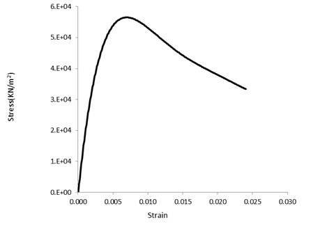
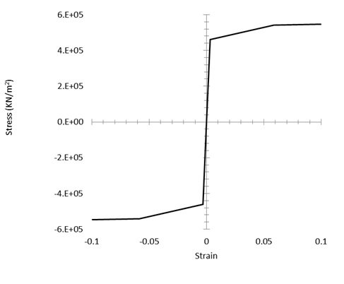
In this model, the cross-section of each fiber element is discretized into vertical concrete and steel fibers. The constitutive law for the nonlinear concrete fibers is based on a confined concrete stress-strain relationship, following a modified Mander model [71], which neglects the tensile strength of concrete. The model incorporates expected material strengths, with the concrete compressive strength taken as 1.3 times its nominal design value and the steel reinforcement yield strength set at 1.17 times its nominal yield strength [72]. The stress-strain curves for the steel reinforcement and the concrete in compression are provided in Figures 10 and 11, respectively.
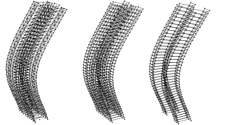
To account for cyclic degradation, the RC wall elements include a degradation factor for the longitudinal reinforcement, defined by the ratio of the area of a degraded hysteresis loop to its non-degraded counterpart [73]. A single element was used to model each RC wall component per story [65]. A perspective view of the complete numerical models prepared for the Nonlinear Time History Analysis (NLTHA) is shown in Figure 12.
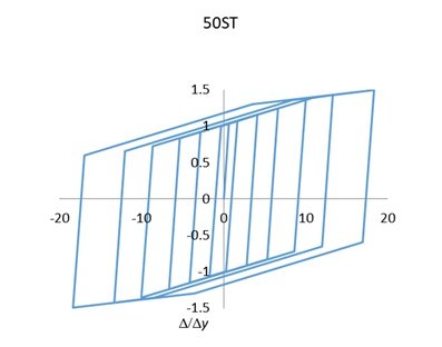
The shear behavior of the wall elements was modeled as linear elastic. The shear stiffness was assigned a value of \(G_cA_g/15\), where \(G_cA_g\) represents the elastic shear stiffness. This value falls within the range of \(G_cA_g/20\) to \(G_cA_g/10\), as recommended by ATC-72. Finally, the hysteretic response of the BRB element implemented in the nonlinear model of the core system is illustrated in Figure 13.
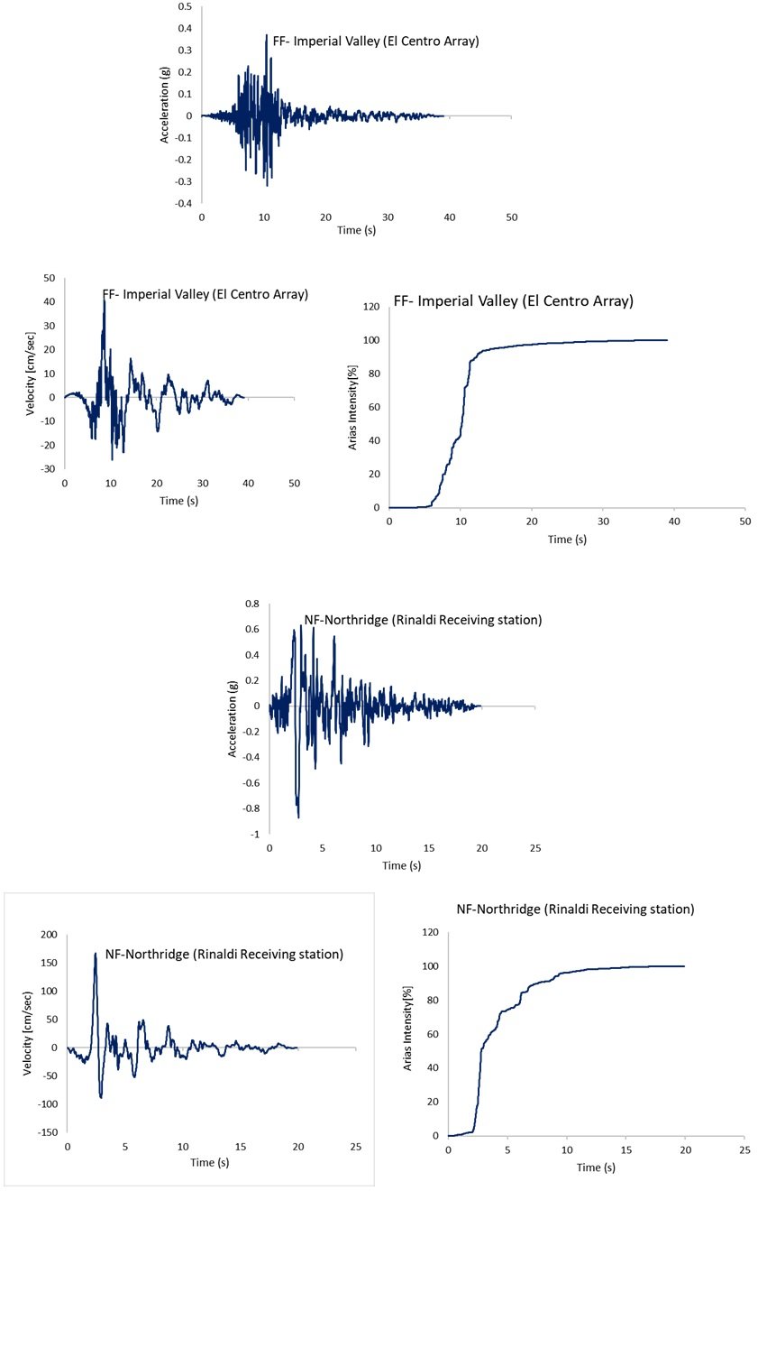
Time history analyses were performed using seismic records to evaluate structural response and energy dissipation during earthquake events. Multiple ground motion records were employed for these dynamic analyses. Near-fault (NF) ground motions exhibit distinctive pulse-like characteristics, typically observed perpendicular to the fault rupture in the fault-normal component. These velocity pulses are most evident in the fault-normal directional components of the ground motion [41].
Figure 14 presents representative acceleration and velocity time histories along with the Arias intensity (Ia) for both near-fault and far-fault records. The Arias intensity, which serves as an indicator of the total energy content in a ground motion record, is calculated using Eq. (2) and provides a reliable measure of seismic destructiveness potential:
\[\label{eq2} I_{a} = \frac{\pi}{2g} \int_{0}^{t_{f}} [a(t)]^{2} dt,\tag{2}\] where \(g\) represents gravitational acceleration, \(t_f\) denotes the total ground motion duration, and \(a(t)\) is the acceleration time history. In near-fault events, the Arias intensity demonstrates a rapid increase that coincides with the occurrence of velocity pulses. These NF motions typically contain significant high-frequency content and may include fling-step effects. Among the various NF characteristics, directivity pulses hold the greatest significance for structural engineering applications.
The study utilized two sets of ground motions: 14 near-fault pulse-like records and 14 ordinary far-fault records, selected from Tables A-6A and A-4A of FEMA P695 [74], respectively. All time histories were obtained from the PEER NGA database, with only the fault-normal components used in the analysis. Complete details of the seismic records are provided in Table 3.
| Event name | Year | Record length (s) |
Station | PGA (g) | M | Site source distance(km) |
|
|---|---|---|---|---|---|---|---|
| Near-Fault record | Imperial valley-06 | 1979 | 39 | El centro Array\#6 | 0.44 | 6.5 | 27.5 |
| Imperial valley-06 | 1979 | 37 | El centro Array\#7 | 0.46 | 6.5 | 27.6 | |
| Irpinia. Italy-01 | 1980 | 40 | Sturno | 0.31 | 6.9 | 30.4 | |
| Superstition-hills-02 | 1987 | 22.3 | Parachute test site | 0.42 | 6.5 | 16 | |
| Loma Prieta | 1989 | 40 | Saratoga-Aloha | 0.38 | 6.9 | 27.2 | |
| Erizican-Turkey | 1992 | 20.8 | Erizican | 0.49 | 6.7 | 9 | |
| Cape Mendocino | 1992 | 36 | Petrolia | 0.63 | 7 | 4.5 | |
| Landers | 1992 | 48 | Lucerne | 0.79 | 7.3 | 44 | |
| Northridge-01 | 1994 | 20 | Rinaldi Receiving Sta | 0.87 | 6.7 | 10.9 | |
| Northridge-01 | 1994 | 40 | Sylmar-Olive View | 0.73 | 6.7 | 16.8 | |
| Kocaeli/IZT | 1999 | 30 | Izmit | 0.22 | 7.5 | 5.3 | |
| Chi chi, Taiwan | 1999 | 90 | TCU065 | 0.82 | 7.6 | 26.7 | |
| Chi chi, Taiwan | 1999 | 90 | TCU102 | 0.29 | 7.6 | 45.6 | |
| Duzce | 1999 | 26 | Duzce | 0.52 | 7.1 | 1.6 | |
| Far-Fault record | Northridge | 1994 | 20 | Canyon Country-WLC | 0.48 | 6.7 | 26.5 |
| Duzce | 1999 | 56 | Bolu | 0.82 | 7.1 | 41.3 | |
| Hector Mine | 1999 | 45.3 | Hector | 0.34 | 7.1 | 26.5 | |
| Imperial valley | 1979 | 100 | Delta | 0.35 | 6.5 | 33.7 | |
| Imperial valley | 1979 | 39 | El centro Array\#11 | 0.38 | 6.5 | 29.4 | |
| Kobe, Japan | 1995 | 41 | Shin- Osaka | 0.24 | 6.9 | 46 | |
| Kocaeli, Turkey | 1999 | 27.2 | Duzce | 0.36 | 7.5 | 98.2 | |
| Kocaeli, Turkey | 1999 | 30 | Arcelik | 0.22 | 7.5 | 53.7 | |
| Landers | 1992 | 44 | Yermo Fire Station | 0.24 | 7.3 | 86 | |
| Loma Prieta | 1989 | 40 | Gilroy Array | 0.56 | 6.9 | 31.4 | |
| Superstition Hills | 1987 | 40 | El Centro lmp. Co. | 0.36 | 6.5 | 35.8 | |
| Superstition Hills | 1987 | 22.3 | Poe Road (temp) | 0.45 | 6.5 | 11.2 | |
| Chi chi, Taiwan | 1999 | 90 | Chy101 | 0.44 | 7.6 | 32 | |
| San Fernando | 1971 | 28 | LA-Hollywood Stor | 0.21 | 6.6 | 39.5 |
Following LATBSDC guidelines, records were scaled to the Maximum Considered Earthquake (MCE) level [72]. Proper scaling methodology is crucial for preparing appropriate acceleration time histories for dynamic analysis [75]. The MCE spectrum was defined as 1.5 times the Design Basis Earthquake (DBE) response spectrum [56]. Scaling was implemented such that the average 5% damped response spectrum across the period range of 0.2T to 1.5T (where T represents the fundamental vibration period) exceeded the MCE spectrum [56]. Figure 14 illustrates the average scaled spectra for both the near-fault and far-fault record sets.
The damping coefficient plays an critical role in shaping structural response during NLTHA [76]. For this study the analysis was completed using Perform-3D, which allows for Rayleigh and modal damping schemes. The software’s documentation indicates that a hybrid strategy may be used based on leveraging the strengths of both approaches [66]. As such a hybrid damping methodology has been implemented-principally utilizing a modal damping formulation with a light coating of Rayleigh damping to control the high frequency components of response.
The Rayleigh formulation requires the choice of two modal frequencies, usually the first mode and another mode where the cumulative mass participation exceeds 90% of the total mass of the system. All the modes were set to a uniform modal damping ratio of 2.5%, as recommended in the software, while Rayleigh damping was set at 0.15%, anchored around the first and the third vibrational modes [66].
Uang and Bertero [49] identified two main methods for calculating earthquake input energy: one based on absolute and the other on relative displacement. Although the choice of a method might affect some analysis details, its influence on the estimation of damage is in general not significant. This is due to the fact that the inelastic part of the energy-the most indicative parameter of the structural damage-is almost insensitive to the method used for its calculation [53].
In this research, the relative displacement approach is used as guided by Chopra [77] and Bruneau and Wang [78]. This choice is in line with the fact that internal forces of the structure originate from the relative displacements and velocities rather than from the absolute ground motion [53].
The governing equations of motion for a structural system with \(N\) degrees of freedom can be formulated as: \[\label{eq3} F_i(t)+F_d(t)+F_s(t)=-Mr{\ddot{u}}_g\left(t\right),\tag{3}\] here, \(F_i\) denotes the inertia force vector, \(F_d\) refers to the damping force vector, and \(F_s\) represents the nonlinear restoring force vector. The mass matrix is denoted by \(M\), the influence vector by \(r\), and \(\ddot{u}_g\) stands for ground acceleration.
During an earthquake, the amount of energy a structure absorbs can vary significantly—shaped by a mix of site-specific conditions, the building’s configuration, and the characteristics of the seismic input, particularly its frequency content. This incoming energy leads to both elastic and inelastic responses across structural elements, depending on how it’s distributed and dissipated.
By transposing Eq. (3) and multiplying through by the differential displacement \(du = \dot{u}dt\), an expression for energy balance can be derived through integration:
\[\label{eq4} \int^u_0{F^T_i(t)}du+\int^u_0{F^T_d}(t)du+\int^u_0{F^T_s\left(t\right)}du=-\int^u_0{M}r{\ddot{u}}_g(t)du,\tag{4}\] where \(u\) represents the relative displacement vector. The terms from left to right correspond to: kinetic energy (\(E_k\)), damping-dissipated energy (\(E_d\)), and internal energy comprising both elastic strain energy (\(E_{el}\)) and inelastic hysteretic energy (\(E_{ine}\)). Structural damage manifests when deformations progress into the inelastic regime. The right-hand term represents the total relative input energy (\(E_i\)).
Eq. (5) summarizes the energy equilibrium relationship, demonstrating that seismic input energy balances with the other energy components at any given time:
\[\label{eq5} E_k+E_d+(E_{el}+E_{ine})=E_i.\tag{5}\]
The nonlinear time history analyses were conducted by utilizing a mix of NF and FF ground motion records. For each case, the relevant energy components as described above were computed. Representative NF and FF events are shown in Figures 15 and 16, respectively, demonstrating the variation of those energy components with time. The Imperial Valley earthquake recorded at the El Centro Array station is considered to represent a typical FF case, and the Northridge earthquake recorded at the Rinaldi Receiving station is taken as representative of NF conditions. In both plots, time is plotted along the horizontal axis, and the energy values are normalized by the total input energy, \(E_i\), along the vertical axis, showing the contribution of each type over the duration of the seismic response.
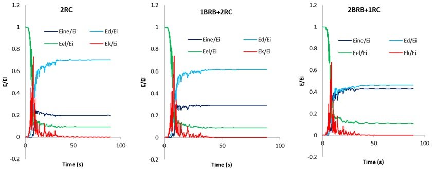
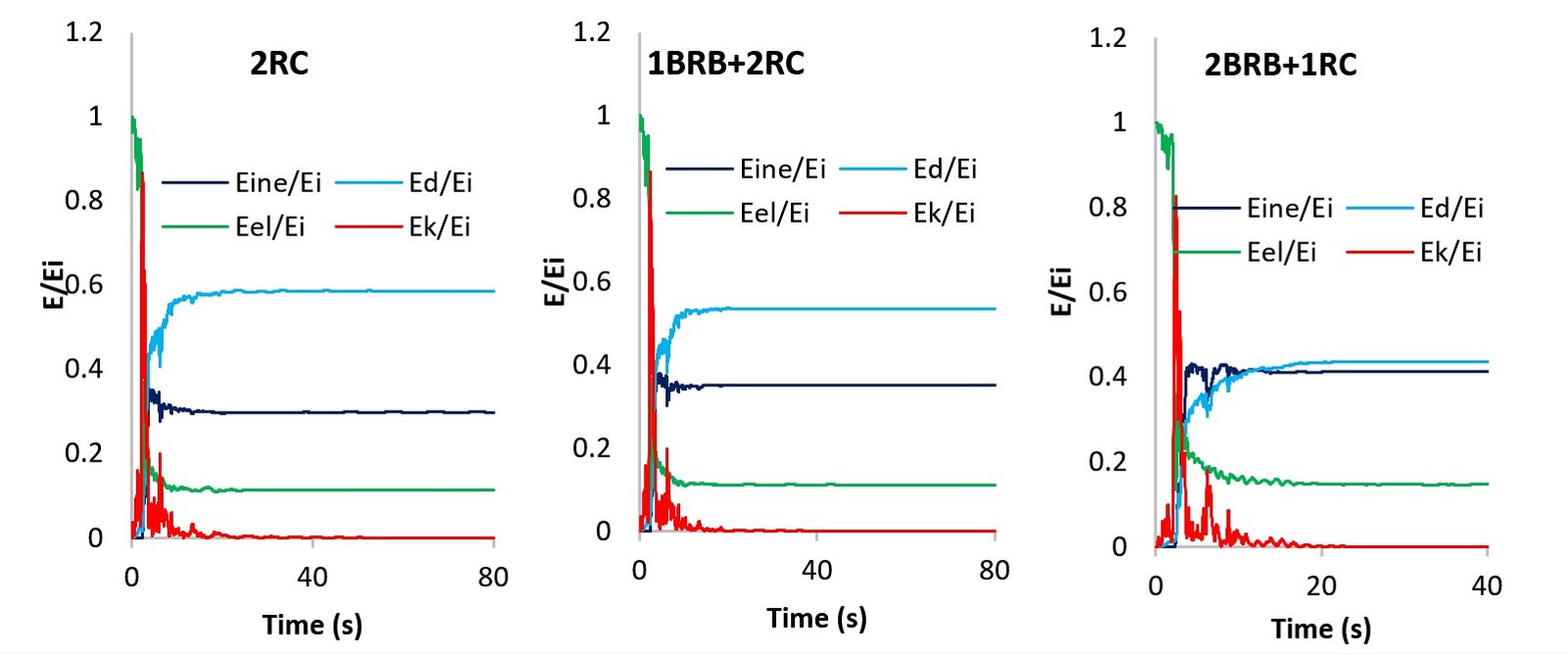
To gain an insight into these dynamics, energy response ratios—\(E_{ine}/E_i\), \(E_k/E_i\), \(E_d/E_i\), and \(E_{el}/E_i\)—are plotted separately for the 2BRB+1RC, 1BRB+2RC, and 2RC configurations. In the initial stages of motion, during which the structural response remains mostly in the linear range, the ratios \(E_{el}/E_i\) and \(E_k/E_i\) maintain relatively high values. When the shaking develops in intensity, these components start to split, following the inverse relation as typically observed for elastic vibrational systems. By the time nonlinear deformations occur, both \(E_{el}/E_i\) and \(E_k/E_i\) fall significantly, a clear indication of the shift to inelastic and damping mechanisms dominating the energy absorption.
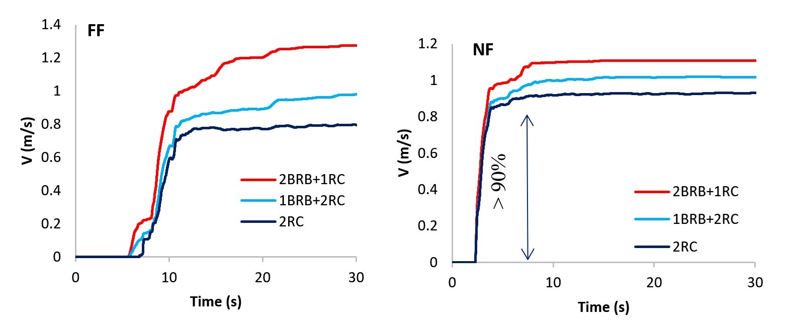
Figure 17 presents a comparison of input energy demand across different structural systems subjected to representative near-fault (NF) and far-fault (FF) earthquake records. The vertical axis indicates the normalized height of the structure, while the horizontal axis reflects the equivalent velocity (\(V\)), a parameter linked to energy (\(E\)) and seismic mass (\(M\)), defined by:
\[\label{eq6} V = \sqrt{\frac{2E}{M}}.\tag{6}\]
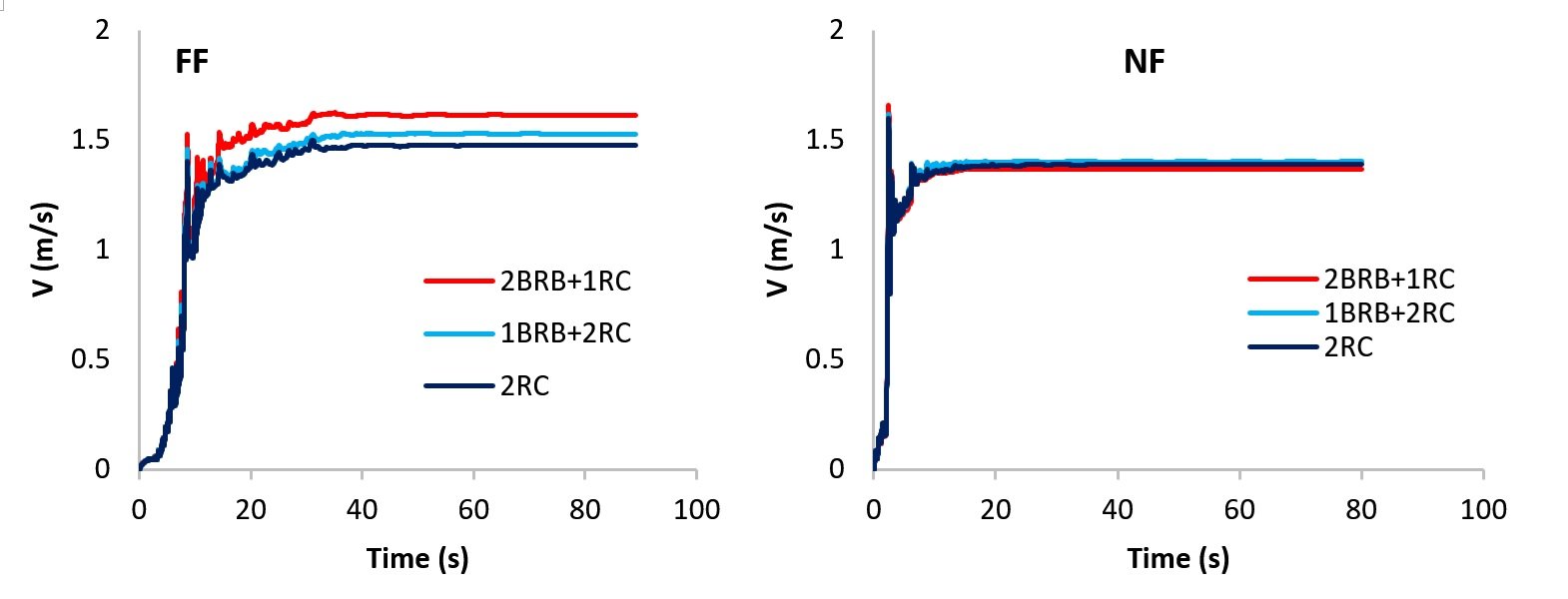
This equivalent velocity is a good proxy for comparing the energy input imparted to a structure. From the figure, it can be seen that no configuration consistently has the highest or lowest input energy for all the events studied; this is partly because the ground motion characteristics, such as frequency content and pulse duration, vary. In all three systems studied here under the NF scenario, the peak energy demand occurs when the velocity pulse arrives, which, for the record shown here, happens close to 2.5 seconds. In that instant the instantaneous energy demand momentarily exceeds the final cumulative input energy, \(E_i\), which generally combines the damping and inelastic energy contributions. This can be seen from the pulse arrival time in the velocity time history (Figure 5) compared to the steep rise in the \(E_i\) curve.
In contrast to NF motions, FF motions do not exhibit sharp velocity pulses and tend to have a more uniform energy accumulation during shaking. Accordingly, peak energy demands may occur toward the end rather than during the early part of an event. Note that overall sharp energy spikes in NF situations typically correspond to those cases when a velocity pulse is caused by an integrated acceleration pulse, not necessarily by multiple high acceleration peaks without an integrated pulse 48.
The energy time histories of Figure 17 illustrate that the demand patterns are a function of a combination of ground motion inputs as well as structural system behavior. Structural vulnerability is strongly related to the peak inelastic energy input during earthquakes. Figure 18 shows the cumulative inelastic energy demands for all configurations due to selected NF and FF records. Of these, the 2BRB+1RC system had the largest demand for most of the individual cases. Similar to total input energy, the amplitude of inelastic demand is controlled by a variety of factors, including the specific characteristics of the earthquake, as well as by the structural configuration. Overall, the average trends in inelastic energy are uniform between NF and FF records, increasing steadily due to its cumulative nature and peaking towards the end of shaking. However, NF events often produce an instantaneous increase in inelastic demand upon the arrival of the velocity pulse, which demonstrates their capacity to generate significant damage.
The findings of this study highlight distinct contrasts in how structures absorb energy during near-fault (NF) versus far-fault (FF) seismic events. On average, structures required roughly 3.5 times longer to absorb 90% of their total inelastic energy under FF motions compared to NF scenarios. A closer look at the data reveals that more than 90% of inelastic energy demand is concentrated in the structure’s first yield excursion. This front-loaded energy input during NF events greatly amplifies the potential for severe structural damage, particularly when high demands are imposed within very short durations.
Figure 19 shows the time histories of damping energy dissipation for each structural system under representative NF and FF ground motions. Under FF loading, the 2BRB+1RC configuration recorded the lowest levels of damping energy, a result likely influenced by the inherent damping behavior of reinforced concrete. In contrast, during NF events, a sharp increase in damping energy is observed as the velocity pulse strikes the structure—highlighting the strong dependence of damping on relative velocity. Such a surge is notably absent in FF cases, where energy dissipation unfolds more steadily across the duration of shaking.
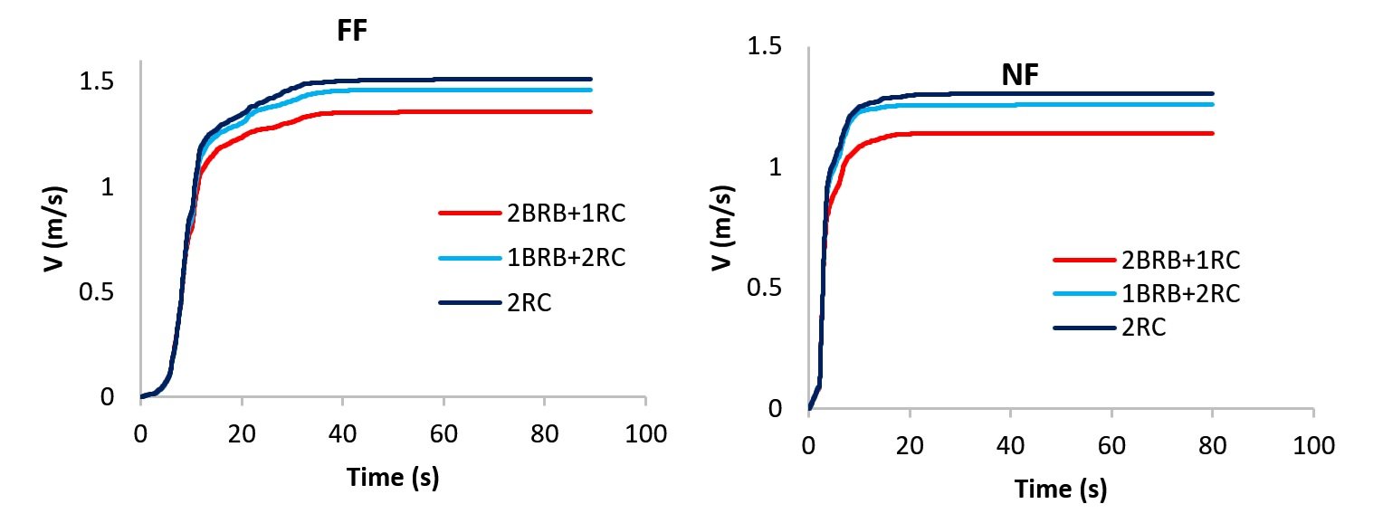
Figure 20 illustrates the time histories of kinetic energy demand for the evaluated structural systems under selected near-fault (NF) and far-fault (FF) earthquakes. The results indicate that NF events tend to generate sharp spikes in kinetic energy, which coincide with the arrival of the velocity pulse. Such abrupt impulses are largely absent in FF records, where kinetic energy accumulates more progressively over time. Interestingly, the kinetic energy demand trends remain largely consistent across all structural configurations subjected to the same ground motion. This consistency stems from the similarity in interstory velocity responses among the systems and reflects the direct dependence of kinetic energy on mass and velocity in structural dynamics.
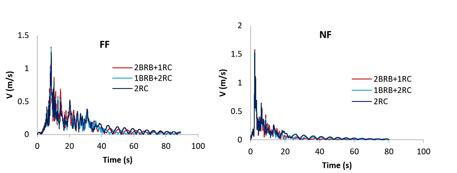
Figure 21 presents the temporal evolution of elastic energy demand under the same seismic scenarios. Much like the kinetic energy trends, NF events produce a sudden increase in elastic energy during the initial pulse phase. However, once the structure yields and enters the nonlinear deformation range, the stored elastic energy quickly dissipates and gradually tapers off. Notably, the elastic energy responses of the 1BRB+2RC and 2RC systems align closely across all examined ground motions, suggesting that the addition of a single buckling-restrained brace does not significantly alter the elastic energy behavior of the overall system.
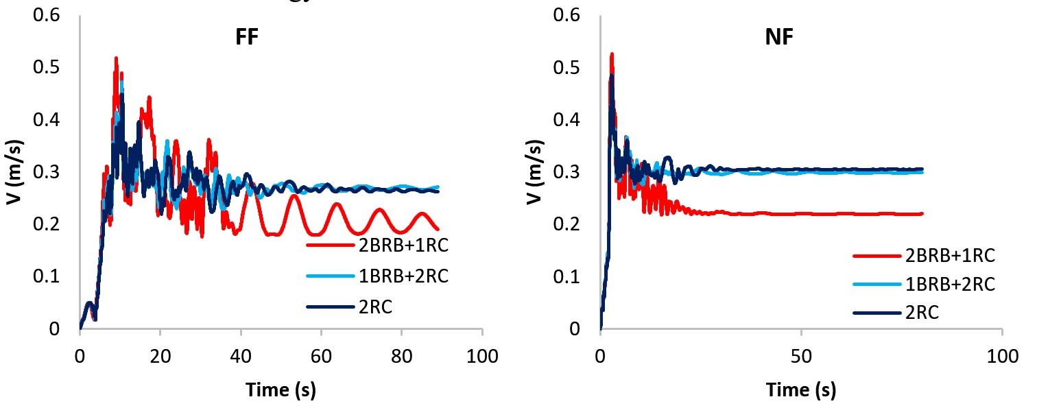
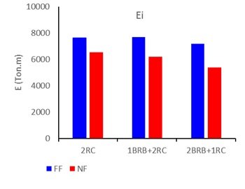
Figure 22 compares the cumulative total input energy—defined as the sum of damping and inelastic energy components measured at the end of structural shaking—for both near-fault (NF) and far-fault (FF) ground motion records. Across all three structural configurations (1BRB+2RC, 2BRB+1RC, and 2RC), NF events consistently resulted in lower total input energy levels than their FF counterparts. This contrast largely reflects key differences in ground motion characteristics, particularly in the duration and frequency content of seismic excitation.
Further insights are offered in Figure 23, which displays the average inelastic energy demands at the conclusion of shaking for all records. The analysis shows that NF earthquakes produce approximately 20–25% less inelastic energy than FF events across all structural systems. This reduction appears consistently across configurations, underscoring a uniform trend in how NF conditions affect energy absorption in the inelastic range.

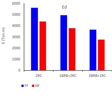
Finally, Figure 24 presents a comparison of average damping energy dissipation between NF and FF cases at the end of the structural response. The results indicate that, on average, damping energy under NF excitations is about 80% of the values recorded for FF events. This ratio holds steady across all three systems, suggesting a systematic decrease in damping dissipation capacity when subjected to near-fault seismic loading.
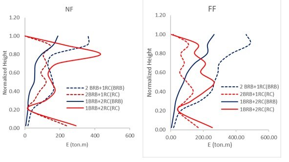
Comparison between NF and FF records effect pertaining to average inelastic energy demand along the height for three approaches is illustrated in Figure 25. The vertical axis represents normalized height of the structure and the horizontal axis shows the inelastic energy demand. Besides, in all examined models, the inelastic energy dissipation at higher levels is larger than the inelastic energy dissipation at the base level that shows larger plasticity at higher levels. The most inelastic energy demand belong to 2BRB+1RC approach that happens at around 0.85H.
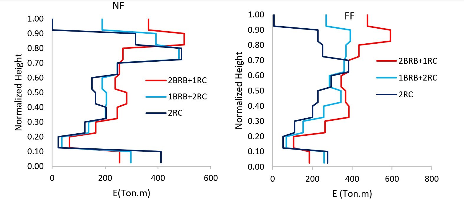
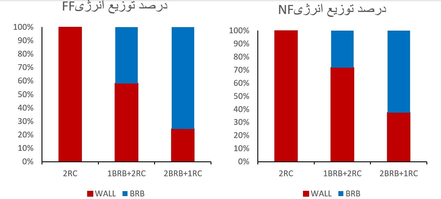
Figure 26 shows the contribution of RC walls and BRBs in inelastic energy absorbed for 1BRB+2RC, 2BRB+1RC and RC models. In the 2BRB+1RC approach, on average for the total FF events, it is obvious that more than 75 percent of inelastic energy, is absorbed by BRBs and for the total NF events this value is approximately 65%. In 1BRB+2RC approach subjected to FF and NF record sets, the contribution of BRBs in inelastic energy demand is 45% and 30%, respectively.
For the combined models, contribution of the RC wall and BRBs in inelastic energy demands along the height has been plotted in Figure 27. In the 2BRB+1RC approach, the contribution of the BRBs above 0.2H is larger than the RC wall and this issue is revers below 0.2H. The reason is the wall stiffness near the base that lead to carry large force and plasticity. In the 1BRB+2RC approach, the main inelastic energy is absorbed by the RC wall, but this matter is reversed above 0.8H for the FF record set.
This study investigated the energy dissipation behavior of tall reinforced concrete core-wall systems integrated with buckling-restrained braced frames under severe seismic loading. Configurations included 2BRB+1RC, consisting of two I-shaped BRBFs with one I-shaped RC wall, and 1BRB+2RC, having one I-shaped BRBF with two I-shaped RC walls, as well as a code-compliant 2RC benchmark without BRBFs. All systems were designed based on prescriptive codes and nonlinearly modeled using fiber elements for RC walls and other proper nonlinear elements for BRBFs. Nonlinear time history analyses were conducted under near-fault forward-directivity and far-fault records, tracking the kinetic, elastic strain, inelastic, and damping energy components.
Results showed a strong dependence of the inelastic energy distribution on system configuration. In the 2BRB+1RC model, BRBFs absorbed around 75% (FF) and 65% (NF) of the total inelastic energy, while in the 1BRB+2RC system they contributed 45% (FF) and 30% (NF). In all models, maximum inelastic energy demand concentrated around 0.8 times the height of the building, reflecting plastic deformation predominantly in upper stories. Compared across record types, NF motions resulted in lower total energy demands: on average, inelastic, damping, and input energies from NF motions were about 80% of those from FF motions. However, NF earthquakes delivered this energy more abruptly; the time to reach 90% of inelastic energy under FF records was roughly 4.5 times under NF records, which reflects the intense, short-duration pulses of NF ground motions.
Abstract Electrical measurements are among the earliest physical measurements carried out by man. As early as 600 BC, the Greek philosopher Thales of Miletus recorded that amber, on being rubbed with fur, becomes electrified. Since then, the study of electricity has continuously grown with experimentation done by several scientists. The discovery of the electron in 1897 by J.J. Thomson marked the beginning of a new era in electrical measurements \(E_k/E_i\) and \(E_{el}/E_i\). It showed strong oscillations in the early, predominantly elastic response—especially for NF motions—but these indeed diminished after yielding, as an increasing fraction of the input energy was channeled into inelastic deformation and damping, rather than remaining in kinetic or elastic strain energy.