

Under dynamic loading conditions, such as earthquakes or impacts, reinforced concrete structures exhibit mechanical behaviors that differ fundamentally from those observed under static loading during the service life. This discrepancy primarily stems from the multidimensional and random characteristics of dynamic loads, together with structural asymmetry, which collectively subject structural members to complex loading histories involving varying strain rates and axial forces. Extensive studies have demonstrated that strain rate effects play a critical role in governing the mechanical performance of reinforced concrete members [1]. Specifically, increasing strain rates have been shown to enhance the carrying capacity, stiffness, and energy dissipation capacity of beams [2], while simultaneously reducing their deformation capacity [3]. At sufficiently high strain rates, the failure mode of beams may shift from ductile flexural failure to brittle shear failure [4]. For columns, elevated strain rates tend to intensify stiffness degradation [5], whereas in shear walls, higher strain rates generally improve both carrying capacity and energy dissipation capacity [6]. Axial force is another important factor influencing the mechanical behavior of reinforced concrete members [7]. An increase in axial force typically leads to a significant reduction in ductility [8, 9], while simultaneously enhancing the carrying capacity of beam-column joints [10]. Moreover, under elastic–plastic deformation, fluctuating axial forces can further accelerate the degradation of strength and stiffness in such joints [11]. Although the individual effects of strain rate and axial force on reinforced concrete members have been widely investigated, most existing studies have primarily focused on quasi-static behavior, with limited attention paid to dynamic performance. In addition, the coupled effects of varying strain rates and axial forces have not yet been systematically examined. Current research largely concentrates on the dynamic response of isolated structural members, such as beams, columns, or shear walls, under simplified loading conditions. Consequently, the dynamic performance of beam-column joints subjected to complex loading scenarios remains insufficiently understood. Therefore, a comprehensive investigation of the mechanical performance of beam-column joints under combined varying strain rates and axial forces is of significant importance. Such research is essential for achieving accurate performance evaluation and for improving the design and assessment of reinforced concrete structures subjected to seismic and other dynamic actions.
Experimental investigation remains extensively utilized for analyzing the mechanical performance of structural members. While accurate results are achievable through experimental methods, these methods frequently entail time-consuming, costly, and challenging to control test conditions. Consequently, a theoretical approach is adopted to investigate the effects of varying strain rates and axial forces on the mechanical performance of beam-column joint. The analysis is grounded in the restoring force model, which serves as a fundamental basis for the theoretical investigation of structural member performance under cyclic loading [12]. This model effectively captures key mechanical responses, such as strength degradation, stiffness degradation, and pinching effects [13], offering a robust framework for simulating complex dynamic behaviors without the practical constraints inherent in physical testing.
Among diverse restoring force models, curvilinear types demonstrate high accuracy but are characterized by structural complexity that hinders practical application. Consequently, polyline models are more widely adopted in engineering due to their computational efficiency and adequate accuracy [14, 15]. Therefore, considerable research has been dedicated to developing polyline models for predicting the mechanical behavior evolution of beam-column joint. For instance, Yu et al. [16] proposed a flat-topped trilinear model derived through theoretical analysis, which effectively characterized the load-displacement relationship across various loading stages. Nevertheless, the descending branch of the skeleton curve, limiting its accuracy beyond the ultimate load, and assumes a symmetric skeleton curve is neglected in this model, whereas actual member responses frequently exhibit asymmetry [17]. To overcome these limitations, Yu et al. [18] established an asymmetric trilinear model calibrated with experimental data, incorporating an ultimate strength point to represent the descending branch and thereby improving predictive accuracy. However, this model was developed confined to quasi-static loading and a fixed axial force, neglecting the effects of varying strain rates or axial forces, which were critical factors influencing the mechanical behaviors [19]. Following a similar methodology, Pang et al. [20] developed an asymmetric trilinear model via regression analysis. Although external strengthening effects were considered, the influences of varying strain rates and axial forces were overlooked. For further refinement, Xue et al. [21] proposed a quadrilinear model that includes a cracking point and employs normalized parameters, considering the stiffness-improving contribution of the slab. Although this model more accurately simulates the actual loading process compared to trilinear formulations, it similarly neglects varying strain rates and axial forces, while failing to adequately represent pinching behavior in hysteretic curves. To address this specific issue, Zhuang et al. [22] defined multiple inflection and compression points into a quadrilinear model, generating hysteretic curves that align better with experimental observations. However, this model also fails to incorporate the effects of varying strain rates and axial forces. Despite the abundance of restoring force models, an appropriate asymmetric model remains lacking for analyzing beam-column joint mechanical properties under complex dynamic loads characterized by coupled variations in strain rates and axial forces.
In summary, to overcome the lack of an appropriate restoring force model for beam-column joints subjected to dynamic loading, this study proposes an asymmetric rate-dependent restoring force model that explicitly incorporates the coupled effects of varying strain rates and axial forces. Based on the plane-section assumption and the principle of energy equivalence, the model is formulated through strip integration combined with parametric analysis and the mean value theorem. The proposed model is subsequently implemented within a finite element framework to evaluate and predict the dynamic performance of beam-column joints under combined variations in strain rates and axial forces.
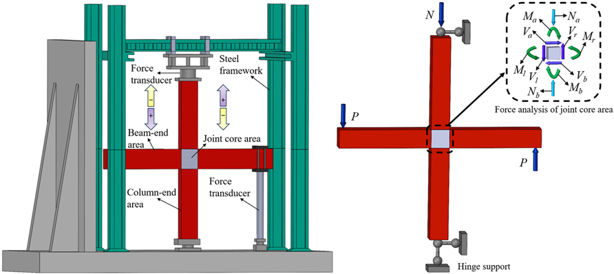
In reinforced concrete frame structures, a beam-column joint is inherently a three-dimensional structural component subjected to complex stress states. To facilitate force analysis and model formulation, the restraining effect of the floor slab is neglected in this study. The beam end and column end are defined as the segments extending from the corresponding inflection points to the joint interface, thereby transforming the spatially complex joint region into an equivalent two-dimensional member within a planar frame system. Based on this simplification, the boundary conditions and force state of the beam-column joint subjected to beam-end loading can be clearly defined. The corresponding mechanical model and force analysis of the simplified joint are illustrated in Figure 1.
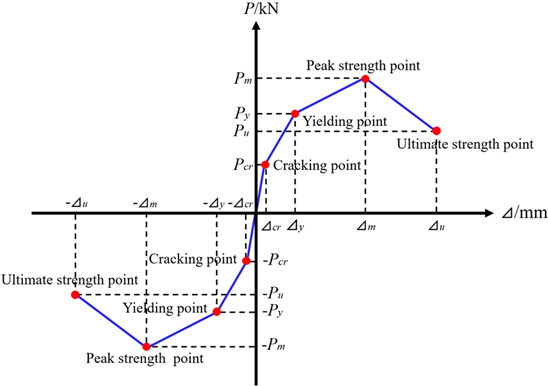
Based on the loading configuration illustrated in Figure 1, the beam-end region is selected as the analytical subject. The loading process at the beam end can be divided into four typical stages: (a) Elastic stage: In this stage, the member stiffness remains constant, and the applied load increases linearly with displacement. This stage terminates at the cracking point, which corresponds to the initiation of concrete cracking and the loss of tensile capacity in the concrete. (b) Elastic-plastic stage: During this stage, the load continues to increase with displacement, but at a reduced rate compared with the elastic stage, resulting in a gradual degradation of stiffness. This stage ends at the yielding point, indicating the onset of reinforcement yielding. (c) Plastic stage: In this stage, the stiffness further decreases relative to the elastic-plastic stage. The load continues to increase until reaching the peak strength point, which signifies that the member has attained its maximum carrying capacity. (d) Failure stage: Beyond the peak strength point, the load begins to decrease while deformation continues to increase until structural failure occurs. This stage concludes at the ultimate strength point. Based on the complete force-deformation characteristics of the beam-column joint, a quadrilinear skeleton curve is established. The skeleton curve is defined by four characteristic points corresponding to cracking, yielding, peak strength, and ultimate strength, as illustrated in Figure 2.
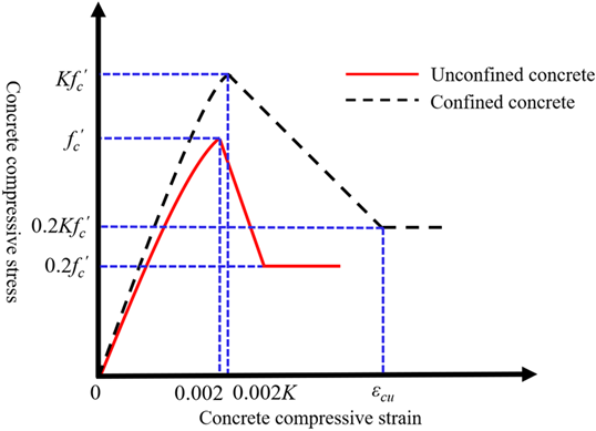
The derivation of load expressions at the characteristic points requires appropriate constitutive models for both reinforcement and concrete. In reinforced concrete members, stirrups are commonly used to enhance structural integrity, as well as to improve the ductility and compressive strength of the core concrete. Therefore, the modified Kent-Park model is adopted in this study as the constitutive model for concrete, since it explicitly accounts for the confinement effect provided by stirrups. The modified Kent-Park model incorporates key parameters related to the strength enhancement of confined concrete, enabling a more realistic representation of concrete behavior under complex loading conditions. By considering the influence of stirrup confinement, this model is well suited for analyzing the mechanical response of beam-column joints subjected to dynamic loading. The constitutive relationship of the modified Kent-Park model is illustrated in Figure 3, and its mathematical expression [23] is given as follows:
\[K = 1 + \frac{\rho_s f_{yh}}{f_c'}, \label{eq1} \tag{1}\]
\[Z_m = \frac{0.5}{ \left(3 + 0.29 f_c'\right)\big/\left(145 f_c' – 1000\right) + 0.75 \rho_s \sqrt{\frac{h''}{s_h}} – 0.002K}, \label{eq2} \tag{2}\]
\[\sigma_c = \begin{cases} K f_c' \left[ \dfrac{2\varepsilon_c}{0.002K} – \left(\dfrac{\varepsilon_c}{0.002K}\right)^2 \right], & 0 \le \varepsilon_c \le 0.002K, \\[8pt] K f_c' \left[1 – Z_m(\varepsilon_c – 0.002K)\right], & 0.002K < \varepsilon_c \le \varepsilon_{cu}, \\[8pt] 0.2K f_c', & \varepsilon_c > \varepsilon_{cu}, \end{cases} \label{eq3} \tag{3}\] where \(\sigma_c\) is the compressive stress of concrete; \(\varepsilon_c\) is the compressive strain of concrete; \(f'_c\) is the cylinder compressive strength of concrete, taken as \(79\%\) of the cubic compressive strength; \(K\) is the strength enhancement factor of confined concrete; \(Z_m\) is the slope of the strain-softening branch; \(\varepsilon_{cu}\) is the ultimate compressive strain of concrete; \(\rho_s\) is the volumetric ratio of stirrup; \(f_{yh}\) is the yield strength of stirrup; \(h''\) is the concrete core width (core area width); and \(S_h\) is the spacing of stirrups.
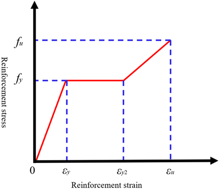
Under dynamic loading conditions, increasing strain rates shorten the yield plateau of reinforcement compared with static loading. In addition, the strain-hardening behavior of reinforcement after yielding plays an important role in governing the mechanical performance of structural members. Therefore, the constitutive model adopted for reinforcement should be capable of accurately describing its post-yield response. In this study, a trilinear elastic-plastic constitutive model with linear hardening is adopted for the reinforcement. This model introduces an ascending branch beyond the yield plateau, enabling an effective representation of the evolution of mechanical behavior after yielding, while maintaining simplicity and computational efficiency. The constitutive relationship of the reinforcement is illustrated in Figure 4, and the corresponding expression [24] is given as follows: \[\label{eq4} \sigma_s= \begin{cases} E_s\,\varepsilon_s, & \varepsilon_s \le \varepsilon_y,\\[2pt] f_y, & \varepsilon_y < \varepsilon_s \le \varepsilon_{y2},\\[2pt] f_y + k\left(\varepsilon_s-\varepsilon_{y2}\right), & \varepsilon_s > \varepsilon_{y2}, \end{cases} \tag{4}\] where \(E_s\) is the elastic modulus of the reinforcement; \(f_y\) is the yield strength of the reinforcement; \(k\) is the strain-hardening ratio and is taken as \(0.01E_s\); \(\varepsilon_s\) is the strain of the reinforcement; \(\varepsilon_y\) is the yield strain of the reinforcement; \(\varepsilon_{y2}\) is the strain at the onset of the strengthening stage; \(\varepsilon_u\) is the ultimate strain of the reinforcement; \(f_u\) is the ultimate strength of the reinforcement.
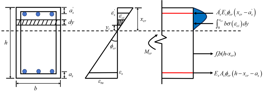
As illustrated in Figure 5, based on the constitutive models for reinforcement and concrete described above, the load expression at the cracking point is derived using strip integration.
The ultimate tensile strain of concrete \(\varepsilon_{tu}\) is expressed as: \[\varepsilon_{tu}=\frac{f_t}{0.5E_c}, \label{eq5} \tag{5}\] where \(f_t\) is the tensile strength of concrete, and \(E_c\) is the elastic modulus of concrete.
The cracking curvature \(\phi_{cr}\) is expressed as: \[\phi_{cr}=\frac{\varepsilon_{tu}}{h-x_{cr}}, \label{eq6} \tag{6}\] where \(h\) is the section depth, and \(x_{cr}\) is the depth of compression zone at cracking.
The compressive strain \(\varepsilon_{ci}\) of concrete strip is expressed as: \[\varepsilon_{ci}=\phi_{cr}\cdot y_i=\frac{\varepsilon_{tu}}{h-x_{cr}}\cdot y_i, \label{eq7} \tag{7}\] where \(y_i\) is the distance from the concrete strip to neutral axis.
Based on the above definitions, the following equilibrium equations are obtained from static equilibrium. \[(x_{cr}-a_s')\cdot\phi_{cr}\cdot E_s\cdot A_s' +\int_{0}^{x_{cr}} b\cdot\sigma_c(\varepsilon_{ci})\,dy =(h-x_{cr}-a_s)\cdot\phi_{cr}\cdot E_s\cdot A_s +f_t\cdot b\cdot(h-x_{cr}), \label{eq8} \tag{8}\]
\[\begin{aligned} \label{eq9} M_{cr} &= \int_{0}^{x_{cr}} b\cdot\sigma_c(\varepsilon_{ci}) \left(y_i+\frac{h-x_{cr}}{2}\right)\,dy +(x_{cr}-a_s')\cdot\phi_{cr}\cdot E_s\cdot A_s' \left(x_{cr}-a_s'+\frac{h-x_{cr}}{2}\right) \notag\\ &\quad +(h-x_{cr}-a_s)\cdot\phi_{cr}\cdot E_s\cdot A_s \left(\frac{h-x_{cr}}{2}-a_s\right), \end{aligned} \tag{9}\] where \(A_s\) and \(A_s'\) are the cross-sectional area of tensile and compressive reinforcement, respectively; \(\sigma_c(\varepsilon_{ci})\) is the stress of concrete strip determined from the constitutive model; \(b\) is the section width; \(a_s'\) and \(a_s\) are the effective depth to the tensile and compressive reinforcement, respectively.
After solving the equilibrium equations for the cracking moment \(M_{cr}\), the corresponding cracking load \(P_{cr}\) is calculated as: \[P_{cr}=\frac{M_{cr}}{L_b}, \label{eq10} \tag{10}\] where \(L_b\) is the beam-end length.
Following the same procedure used to determine the cracking load \(P_{cr}\), the yielding load \(P_y\) and the peak load \(P_m\) are subsequently determined. The yield strain \(\varepsilon_y\) of tensile reinforcement is expressed as: \[\varepsilon_y=\frac{f_y}{E_s}. \label{eq11} \tag{11}\]
The yield curvature \(\phi_y\) is expressed as: \[\phi_y=\frac{\varepsilon_y}{h-x_y-a_s}, \label{eq12} \tag{12}\] where \(x_y\) is the depth of compression zone at reinforcement yielding.
The compressive strain \(\varepsilon_{ci}\) of concrete strip is expressed as: \[\varepsilon_{ci}=\phi_y\cdot y_i=\frac{\varepsilon_y}{h-x_y-a_s}\cdot y_i. \label{eq13} \tag{13}\]
The corresponding equilibrium equations for determining the yielding load are given as follows: \[E_s\cdot\phi_y\cdot(x_y-a_s')\cdot A_s' +\int_{0}^{x_y} b\cdot\sigma_c(\varepsilon_{ci})\,dy =f_y\cdot A_s, \label{eq14} \tag{14}\]
\[M_y= E_s\cdot A_s'\cdot\phi_y\cdot(x_y-a_s')\cdot(h-a_s-a_s') +\int_{0}^{x_y} b\cdot\sigma_c(\varepsilon_{ci})\cdot(y_i+h-x_y-a_s)\,dy. \label{eq15} \tag{15}\]
After obtaining the yielding moment \(M_y\) from the simultaneous equilibrium equations, the yielding load \(P_y\) can be calculated as: \[P_y=\frac{M_y}{L_b}. \label{eq16} \tag{16}\]
When the concrete strain reaches its peak value, the peak curvature \(\phi_m\) is expressed as: \[\phi_m=\frac{\varepsilon_0}{x_m}, \label{eq17} \tag{17}\] where \(x_m\) is the depth of compression zone at peaking load, and \(\varepsilon_0\) is the peak strain of concrete, taken as 0.002.
The compressive strain \(\varepsilon_{ci}\) of the concrete strip is expressed as: \[\varepsilon_{ci}=\phi_m\cdot y_i=\frac{\varepsilon_0}{x_m}\cdot y_i, \label{eq18} \tag{18}\]
The corresponding equilibrium equations are expressed as: \[E_s\cdot\phi_m\cdot(x_m-a_s')\cdot A_s' +\int_{0}^{x_m} b\cdot\sigma_c(\varepsilon_{ci})\,dy =f_u\cdot A_s, \label{eq19} \tag{19}\] \[M_m= E_s\cdot A_s'\cdot \phi_m\cdot (x_m-a_s')\cdot (h-a_s-a_s') +\int_{0}^{x_m} b\cdot\sigma_c(\varepsilon_{ci})\cdot (y_i+h-x_m-a_s)\,dy. \label{eq20} \tag{20}\]
After obtaining the peaking moment \(M_m\) from the simultaneous equilibrium equations, the peaking load \(P_m\) can be calculated as: \[P_m=\frac{M_m}{L_b}. \label{eq21} \tag{21}\]
The ultimate load \(P_u\) is defined as 0.85 times the peaking load \(P_m\): \[P_u=0.85\,P_m. \label{eq22} \tag{22}\]
During the loading process of a beam-column joint, the member remains in an elastic or elastic–plastic state until reinforcement yielding occurs. Within this stage, variations in stiffness are relatively small and can be neglected. Therefore, based on the plastic hinge theory and considering the contributions of various deformation components to the overall displacement, the beam-end displacement before reinforcement yielding can be calculated as: \[\Delta_b=\frac{\phi}{3}(L_b+0.022\,f_y\,d_b)^2 \left[1+\left(\frac{h}{L_b}\right)^2\right], \qquad \phi\leq\phi_y, \label{eq23} \tag{23}\] where \(\phi\) is the sectional curvature, which is determined based on the beam-end displacement; \(d_b\) is the diameter of longitudinal reinforcement.
After the reinforcement at the beam-end section corresponding to the maximum bending moment yields, the yielded region gradually expands with increasing external load, eventually leading to the formation of a plastic hinge zone. Within this zone, the sectional curvature increases rapidly, resulting in significant rotational deformation at the beam end and a corresponding increase in displacement. Consequently, the influence of the plastic hinge must be considered in the beam-end displacement \(\Delta_p\) after reinforcement yielding. In this stage, the total displacement consists of both elastic and plastic components, as illustrated in Figure 6.
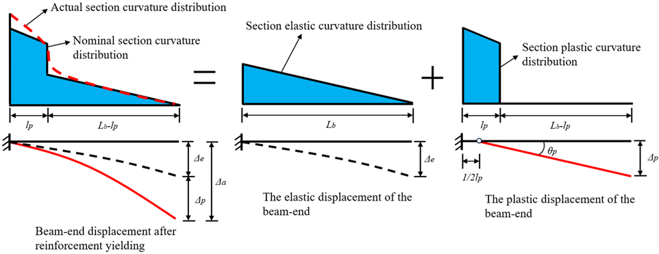
According to the established method for evaluating plastic displacement, the plastic component is primarily governed by the length of the plastic hinge zone. To incorporate the influence of varying axial force into the restoring force model, based on a commonly adopted empirical expression, the formula for calculating the length of the plastic hinge zone \(l_p\), while considering the influence of the axial compression ratio, is expressed as follows: \[l_p=2(h-a_s)\left[1-\frac{0.5(\mu_s f_{yt}-\mu_{sc}f_{yc}+N_1/bh)}{f_c}\right], \label{eq24} \tag{24}\] where \(\mu_{st}\) and \(\mu_{sc}\) are the tensile and compressive reinforcement ratios, respectively; \(f_{yt}\) and \(f_{yc}\) are the yield strengths of the tensile and compressive reinforcement; \(N_1\) is the axial force; \(f_c\) is the compressive strength of concrete.
The plastic displacement \(\Delta_p\) of the beam-end is expressed as: \[\Delta_p=(\phi-\phi_y)\cdot l_p\cdot\left(L_b-\frac{1}{2}l_p\right), \qquad \phi\geq\phi_y. \label{eq25} \tag{25}\]
The elastic displacement \(\Delta_e\) is calculated using the same method as for the displacement \(\Delta_b\) before reinforcement yielding. The total beam-end displacement \(\Delta_a\) after reinforcement yields is expressed as: \[\Delta_a=\Delta_e+\Delta_p =\frac{\phi_y}{3}(L_b+0.022\,f_y\,d_b)^2 \left[1+\left(\frac{h}{L_b}\right)^2\right] +(\phi-\phi_y)\cdot l_p\cdot\left(L_b-\frac{1}{2}l_p\right), \qquad \phi\geq\phi_y. \label{eq26} \tag{26}\]
Based on the above expressions, the displacements corresponding to the characteristic points on the skeleton curve can be obtained by substituting the section curvatures derived previously.
Both reinforcement and concrete are strain rate–sensitive materials, and their mechanical properties exhibit pronounced differences under dynamic and static loading conditions. Therefore, the strain rate effect must be explicitly considered in the development of the restoring force model. In this study, the influence of strain rate is incorporated through the dynamic increase factor (DIF), which is commonly used to quantify variations in material properties under dynamic loading. By introducing DIF, key mechanical parameters are modified relative to their corresponding static values. The formula is as follows: \[f_d=\mathrm{DIF}\cdot f_s, \label{eq27} \tag{27}\] where \(f_d\) and \(f_s\) are the dynamic and static material strengths, respectively.
The Comité Euro-International du Béton (CEB) provides empirical DIF formulations that relate the dynamic material properties to their static counterparts [30]. For the tensile strength \(f_t\) of concrete under dynamic load, the \(\mathrm{DIF}_{f_t}\) formula is expressed as: \[\mathrm{DIF}_{f_t}=\frac{f_{td}}{f_{ts}} =\left(\frac{\dot{\varepsilon}}{\dot{\varepsilon}_0}\right)^{1.016\,\delta}, \label{eq28} \tag{28}\] where \(f_{td}\) is the dynamic tensile strength of concrete; \(f_{ts}\) is the static tensile strength of concrete; \(\dot{\varepsilon}\) is the strain rate; \(\dot{\varepsilon}_0\) is a constant taken as \(30\times10^{-6}\,\mathrm{s}^{-1}\); \(f_{cs}\) is the static compressive strength of concrete; \(f_0\) is a constant equal to \(10\,\mathrm{MPa}\); and \[\delta=\frac{1}{10+6(f_{cs}/f_0)}.\]
For the compressive strength \(f_c\) of concrete under dynamic loading, the \(\mathrm{DIF}_{f_c}\) formula is expressed as: \[\mathrm{DIF}_{f_c}=\frac{f_{cd}}{f_{cs}} =\left(\frac{\dot{\varepsilon}}{\dot{\varepsilon}_0}\right)^{1.026\,\alpha}, \label{eq29} \tag{29}\] where \(f_{cd}\) is the dynamic compressive strength of concrete, and \[\alpha=\frac{1}{5+9(f_{cs}/f_0)}.\]
For the yield strength \(f_y\) of reinforcement under dynamic load, the \(\mathrm{DIF}_{f_y}\) formula is expressed as: \[\mathrm{DIF}_{f_y}=\frac{f_{yd}}{f_{ys}} =1+\frac{6}{f_{ys}}\ln\!\left(\frac{\dot{\varepsilon}}{\dot{\varepsilon}_{0.3}}\right), \label{eq30} \tag{30}\] where \(f_{yd}\) is the dynamic yield strength of reinforcement; \(f_{ys}\) is the static yield strength of reinforcement; and \(\dot{\varepsilon}_{0.3}\) is a constant equal to \(5\times10^{-5}\,\mathrm{s}^{-1}\).
For the ultimate strength \(f_u\) of reinforcement under dynamic load, the \(\mathrm{DIF}_{f_u}\) formula is expressed as: \[\mathrm{DIF}_{f_u}=\frac{f_{ud}}{f_{us}} =1+\frac{6}{f_{us}}\ln\!\left(\frac{\dot{\varepsilon}}{\dot{\varepsilon}_{0.3}}\right), \label{eq31} \tag{31}\] where \(f_{ud}\) is the dynamic ultimate strength of reinforcement; \(f_{us}\) is the static ultimate strength of reinforcement. The effect of strain rate on the elastic modulus of reinforcement and concrete is negligible [30] and is therefore not considered in this model.
The calculation of the DIF for reinforcement and concrete requires the definition of a representative strain rate. According to Reference [29], although the strain rate under dynamic loading varies continuously, significant changes in mechanical performance generally occur only when the strain rate increases by one order of magnitude or more. To account for this characteristic, the strain rate is defined in two distinct stages: an elastic strain rate prior to reinforcement yielding, and a plastic strain rate after reinforcement yielding. This staged definition enables a more realistic characterization of strain rate evolution and thereby improves the predictive accuracy of the restoring force model.
Before reinforcement yielding, the member remains predominantly in an elastic stage, during which the strain rate can be regarded as approximately constant. This elastic strain rate \(\dot{\varepsilon}_1\) can be obtained using the theoretical formula derived from its physical significance. It is expressed as: \[\dot{\varepsilon}_1=\frac{\varepsilon_1}{T_1}, \label{eq32} \tag{32}\] where \(V\) is the loading speed; \(\mathrm{PSD}_1\) is the yield displacement \(\Delta_y\); \(\varepsilon_1\) is the yield strain \(\varepsilon_y\) of the reinforcement; and \[T_1=\frac{\mathrm{PSD}_1}{V}.\]
After reinforcement yielding, a plastic hinge forms at the beam end, resulting in a pronounced difference in strain rate distribution between the plastic hinge zone and the non-plastic hinge zone. In the non-plastic hinge region, the strain rate remains relatively stable and is comparable to that before yielding. In contrast, within the plastic hinge zone, the strain rate varies continuously due to the development of plastic deformation. Owing to the non-uniformity and uncertainty of the strain rate in the plastic hinge zone, the strain rate calculated directly from the theoretical expression tends to be significantly higher than the actual value during this stage. To improve the accuracy of the plastic strain rate, a reduction factor \(\omega\) is introduced. Based on the physical definition of strain rate, \(\omega\) is derived from the relationship between reinforcement strain and beam-end length. First, the actual strain–length variation curve is simplified into a nominal curve using the equivalent area method, as illustrated in Figure 7. Subsequently, according to the principle of energy equivalence, the ratio of the area enclosed by the nominal curve to that of the actual curve is calculated and defined as the reduction factor \(\omega\).
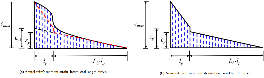
The area enclosed by the strain–length curve represents the length variation. Accordingly, the nominal length increment \(\Delta l\) of the beam can be expressed as: \[\Delta l =\frac{1}{2}\,\varepsilon_y\,(L_b-l_p) +\frac{(\varepsilon_{\max}+\varepsilon_{y1})\,l_p}{2}, \label{eq33} \tag{33}\] where \(\varepsilon_{y1}\) is the nominal yield strain of reinforcement; \(\varepsilon_{\max}\) is the maximum reinforcement strain, \[\varepsilon_{\max}=0.0033\,\frac{(h-a_s-x_u)}{x_u},\] and \(x_u\) is the depth of compression zone at ultimate load.
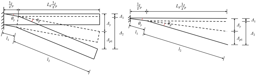
Based on geometrical analysis, the actual length variation \(\Delta l'\) of the beam is calculated from deformation components, including displacement variation and beam-end rotation angle, as illustrated in Figure 8. The first variation length \(l_1\) is expressed as: \[l_1=\sqrt{\frac{1}{4}\,l_p^2+\Delta_1^2}, \label{eq34} \tag{34}\] where \(\theta_y\) is the yield rotation angle, \(\theta_y=\Delta_y/L_b\), and \(\Delta_1=\frac{1}{2}\,l_p\,\theta_y\).
The second variation length \(l_2\) is expressed as: \[l_2=\sqrt{\left(L_b-\frac{1}{2}l_p\right)^2+\Delta_2^2} \label{eq35} \tag{35}\] where \(\theta_p\) is the plastic rotation angle, \[\theta_p=l_p(\phi_u-\phi_y), \qquad \Delta_{p1}=\theta_p\left[L_b-\frac{1}{2}l_p\right], \qquad \Delta_2=\Delta_1+\Delta_{p1}-\Delta_1.\]
The actual length increment \(\Delta l'\) of the beam is expressed as: \[\Delta l'=l_1+l_2-L_b. \label{eq36} \tag{36}\]
The strain-rate reduction factor \(\omega\) \((\omega<1)\) is expressed as: \[\omega=\frac{\Delta l}{\Delta l'}. \label{eq37} \tag{37}\]
The plastic stage strain rate \(\dot{\varepsilon}_2\) is expressed as: \[\dot{\varepsilon}_2=\dot{\varepsilon}_1\cdot\omega=\frac{\varepsilon_1}{T_1}\cdot\omega. \label{eq38} \tag{38}\]
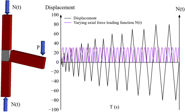
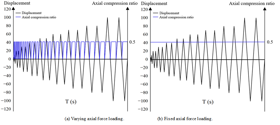
Under dynamic loading, the axial force acting on a beam-column joint varies continuously due to the combined effects of overturning moment and vertical vibration. Previous studies have shown that varying axial force significantly influences mechanical performance indicators such as strength, stiffness, and energy dissipation capacity. Therefore, the effect of varying axial force must be incorporated into the restoring force model. Based on the principle of energy equivalence, the varying axial force is transformed into an equivalent fixed axial force using the mean value theorem. This equivalent fixed axial force \(N'\) is then used in the expressions for the characteristic points of the skeleton curve. The equivalent axial force \(N'\) is expressed as: \[N'=\frac{\displaystyle\int_0^{T}N(t)\,dt}{T}, \label{eq39} \tag{39}\] where \(T\) is the loading time; \(N(t)\) is the time-varying axial force function, determined by the loading protocol, as shown in Figure 9.
Structural members inevitably exhibit asymmetric hysteretic behavior under dynamic loading. This asymmetry primarily arises from factors such as concrete cracking, bond–slip between reinforcement and concrete, and asymmetric reinforcement layout. As a consequence, hysteretic curves derived from symmetric skeleton curves may deviate significantly from the actual structural response. To address this limitation, asymmetry is explicitly incorporated into the skeleton curve when establishing the restoring force model.
Reference [32] proposed an asymmetric BWBN model that incorporated a control parameter \(\delta\) to adjust both the magnitude and direction of the offset of the skeleton curve, thereby effectively capturing asymmetric behavior. Following this approach, the characteristic point parameters are calibrated to account for asymmetry based on the original skeleton curve. The relationship between load and displacement is expressed as follows: \[R(u,z)=\alpha k_0 u+(1-\alpha)k_0 z, \label{eq40} \tag{40}\] where \(R(u,z)\) is the load at the characteristic point; \(k_0\) is the initial elastic stiffness; \(\alpha\) is the post-yield stiffness ratio; \(u\) is the displacement at the characteristic point; and \(z\) is the nonlinear hysteretic displacement.
The maximum nonlinear hysteretic displacement \(z_{\max}\) is expressed as: \[z_{\max}=\left[-\left(1+\delta_v w\right)\left(\beta+\gamma\pm2\delta\right)\right]^{-1/n}, \label{eq41} \tag{41}\] where \(\beta\), \(\gamma\), and \(n\) are shape control parameters; \(\delta\) is the asymmetric control parameter; \(\delta_v\) is the strength degradation parameter; \[w=\int_{0}^{\Delta_u}P(\Delta)\,d\Delta,\] \(P(\Delta)\) is the skeleton curve function; and \(\Delta_u\) is the ultimate displacement.
The control parameters are selected according to the data listed in Table 1. Subsequently, the maximum nonlinear hysteretic displacement \(z_{\max}\) is calculated using Eq. (41). The modified positive and negative peak loads \(P_m\) can be produced by substituting this value into Eq. (40). Thereafter, the loads and displacements at the remaining characteristic points are determined through stiffness-based relationships. This procedure ultimately enables the construction of the asymmetric skeleton curve.
| Parameter | Physical meaning | Parameter distribution range |
|---|---|---|
| \(\alpha\) | Post-yield stiffness ratio | \([0,1.0]\) |
| \(\beta\) | Loading and unloading shape parameters | \([0.5,1.5]\) |
| \(\gamma\) | Loading and unloading shape parameters | \([-0.3,0.5]\) |
| \(n\) | The yield sharpness shape parameter | \([0,5]\) |
| \(\delta_v\) | Strength degradation parameters | \([0,0.05]\) |
| \(\delta\) | Asymmetric control parameters | \([-0.1,0.1]\) |
Under cyclic loading, the unloading stiffness of the member is approximately equal to the elastic stiffness prior to the cracking point. After cracking occurs, however, plastic deformation progressively develops under the combined influence of varying strain rates and axial forces, resulting in a pronounced degradation of unloading stiffness. Therefore, it is necessary to establish an unloading stiffness expression that explicitly accounts for these effects. Based on the relevant research reported in [19], the original unloading stiffness formula is used as a foundation and a multiple regression analysis is conducted on existing test data. Parameters \(a\) and \(c\) related to varying strain rates and axial forces are incorporated to obtain the expression for the unloading stiffness \(K\) after the cracking point: \[\frac{K}{K_0}=a\cdot c^{\Delta/\Delta_i}, \label{eq42} \tag{42}\]
\[a=0.179\,\lg\!\left(\frac{\dot{\varepsilon}}{\dot{\varepsilon}_{0.5}}\right) +0.105\,\lg(1+\bar{n})+1.301, \label{eq43} \tag{43}\]
\[c=0.222\,\lg\!\left(\frac{\dot{\varepsilon}}{\dot{\varepsilon}_{0.5}}\right) -0.317\,\lg(1+\bar{n})+0.378, \label{eq44} \tag{44}\] where \(K_0\) is the elastic stiffness; \(\Delta\) is the member displacement; \(\Delta_i\) is the displacement amplitude of the \(i\)-th loading grade, defined by the loading protocol; \(\bar{n}\) is the rate of change in axial compression ratio; and \(\dot{\varepsilon}_{0.5}\) is a reference strain rate, taken as \(10^{-5}\,\mathrm{s}^{-1}\).
The variation trend of reloading stiffness at different loading stages is generally consistent with that of unloading stiffness. Nevertheless, the influence of varying strain rates and axial forces on the reloading stiffness is relatively small and can be neglected for the sake of computational simplicity. Therefore, the reloading stiffness \(K'\) after the cracking point is calculated using the original model expression. \[\frac{K'}{K}=0.231\left(\frac{\Delta}{\Delta_i}\right)^{-0.979}. \label{eq45} \tag{45}\]
Under cyclic loading, once the member reaches the yielding point, the hysteretic response exhibits pronounced pinching behavior. This phenomenon is mainly attributed to plastic deformation, bond–slip between reinforcement and concrete, as well as the opening and closing of cracks. With increasing displacement and load amplitude, especially beyond the peak load, the pinching effect becomes increasingly significant. Furthermore, an examination of hysteretic curves reported [19] indicates that pinching in beam–column joints under dynamic loading typically initiates near the cracking load. Thus, to accurately simulate this behavior, a damage index \(D\) is incorporated into the loading and unloading stiffness expressions. The introduction of this index induces a stiffness change at the cracking load and generates an inflection point in the hysteretic path, thereby enabling an effective simulation of the pinching effect.
The Park–Ang damage model is widely employed to evaluate structural damage based on cumulative energy dissipation, and thus provides a well-established experimental foundation for calculating the damage index \(D\) [33]. However, the original model does not adequately distinguish failure characteristics under different displacement amplitudes and tends to underestimate the contribution of large-amplitude cycles to the total energy dissipation. To more accurately capture the evolution of loading and unloading stiffness under dynamic loading, the original Park–Ang model is modified by introducing an effective energy dissipation factor \(e_m\), which redistributes the energy dissipation contribution among different displacement amplitudes. The improved Park–Ang model is given by: \[e_m=\frac{\Delta_y}{\Delta_m}\, \log\!\left(\frac{\Delta_u}{\Delta_y}\right) \left(\frac{\Delta_m}{\Delta_y}\right), \label{eq46} \tag{46}\]
\[D=\frac{\Delta_m}{\Delta_u} +e_m\cdot\frac{\sum E_i}{Q_y\,\Delta_u}, \label{eq47} \tag{47}\] where \(\Delta_m\) is the peaking displacement; \[\sum E_i=w=\int_{0}^{\Delta_u}P(\Delta)\,d\Delta,\] \(Q_y=P_y/A\); and \(A\) is the cross-sectional area.
Integrating the damage index \(D\) and the original loading and unloading stiffness expressions, the unloading stiffness \(K_1\) at the inflection point is expressed as: \[K_1=K\cdot(1-D). \label{eq48} \tag{48}\]
The formula for reloading stiffness \(K_1'\) at the inflection point is expressed as: \[K_1'=K'\cdot(1-D). \label{eq49} \tag{49}\]
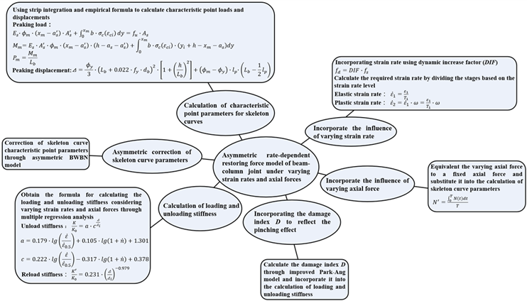
An asymmetric rate-dependent restoring force model for beam-column joints under varying strain rates and axial forces has been established. This model is developed based on the skeleton curve and the degradation rules of loading and unloading stiffness, as illustrated in Figure 10. In addition, the overall theoretical framework of the restoring force model is presented in Figure 11. The hysteretic behavior of the proposed model can be summarized as follows.
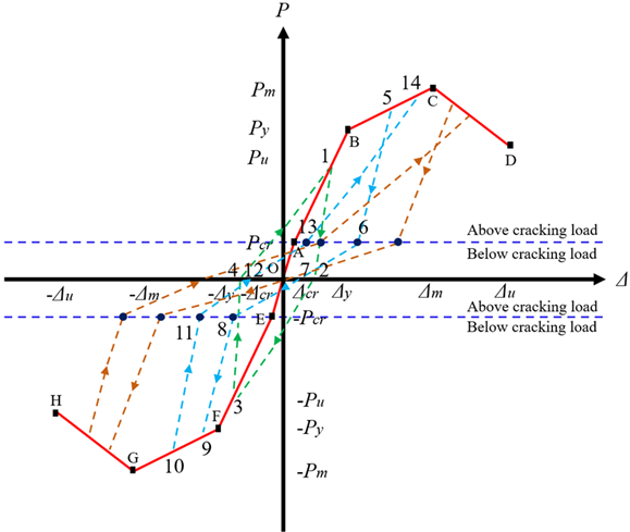
During the cracking stage, both the positive and negative loading–unloading paths follow the skeleton curve, corresponding to segments OA and OE in Figure 10. In this stage, the unloading stiffness and reloading stiffness are equal to the initial elastic stiffness.
When the applied load exceeds the cracking load \(P_{cr}\) and the member enters the yield stage, spanning from the cracking point A to the yielding point B, the initial loading path continues to follow the skeleton curve. However, the unloading path deviates from the original loading path, as indicated by path \(1\rightarrow2\). The unloading stiffness begins to degrade and is calculated using Eq. (42). After unloading to zero load, reverse reloading initiates from the intersection of the unloading path with the coordinate axis. The reloading path follows \(2\rightarrow3\), with the reloading stiffness determined using Eq. (45). Upon reloading to point 3, subsequent unloading and reloading proceed along paths \(3\rightarrow4\) and \(4\rightarrow1\), respectively, forming a closed hysteretic loop. The corresponding stiffness values are consistently calculated using Eqs. (42) and (45). The complete hysteretic path in this stage is \(1\rightarrow2\rightarrow3\rightarrow4\rightarrow1\).
When the applied load further exceeds the yielding point and the member enters the peak stage, spanning from point B to point C, the unloading path is divided into two segments by an inflection point, as shown by path \(5\rightarrow6\rightarrow7\). The unloading stiffness is calculated separately for each segment, with the cracking load serving as the division criterion: Eq. (42) is applied for segment \(5\rightarrow6\), while Eq. (48) is used for segment \(6\rightarrow7\). During reverse reloading, the reloading path also consists of two segments divided by an inflection point, following paths \(7\rightarrow8\) and \(8\rightarrow9\). The reloading stiffness is evaluated separately for each segment, with Eq. (45) applied to segment \(7\rightarrow8\) and Eq. (49) to segment \(8\rightarrow9\). After reloading to point 10, subsequent unloading and reloading follow paths \(10\rightarrow11\rightarrow12\) and \(12\rightarrow13\rightarrow14\), respectively, until a complete hysteretic loop is formed. The stiffness values throughout this process are calculated using the corresponding equations. The complete hysteretic path in this stage is \(5\rightarrow6\rightarrow7\rightarrow8\rightarrow9\rightarrow10\rightarrow11\rightarrow12\rightarrow13\rightarrow14\).
When the applied load exceeds the peak load \(P_m\) and the member enters the ultimate stage, spanning from point C to point D, the hysteretic path exhibits a pattern similar to that observed in the peak stage, as shown in Figure 10.
To validate the proposed restoring force model, a total of 29 experimental datasets obtained from beam-column joint tests [19, 34, 35] are utilized for comparison with model predictions. The model performance is evaluated from multiple perspectives, including the skeleton curve, hysteretic behavior, displacement ductility factor, secant stiffness, cumulative energy dissipation, and equivalent viscous damping coefficient. The key information of the selected beam-column joint specimens is summarized in Table 2.
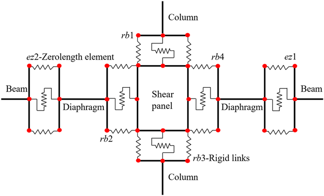
Incorporating the restoring force model proposed in section 3, a finite element model of the beam–column joint is developed in OpenSees to predict its dynamic mechanical performance. In the numerical model, the “Concrete02” and “Steel02” material models are employed to represent the constitutive behavior of concrete and reinforcement, respectively. The joint shear panel is depicted through four “RigidLink” commands (denoted as rbi, \(i=1\)–4), which ensure the rigid connection within the panel. The beam-end is connected to the shear panel via “ZeroLength” elements (\(ezi\), \(i=1,2\)), enabling precise simulation of the connection behavior. To reproduce the hysteretic response of the beam–column joint, the “Pinching4” material model is adopted. The parameters of this material are calibrated based on the proposed restoring force model, including the characteristic points of the skeleton curve, the loading and unloading stiffness, and the damage indices. The overall finite element model configuration is illustrated in Figure 12.
| Research team | Specimen | Sectional dimension \(b\times h\) (mm) |
Length (mm) |
Longitudinal reinforcement ratio (\%) |
Transversal reinforcement ratio (\%) |
Strain rate | Axial compression ratio |
|
|---|---|---|---|---|---|---|---|---|
| Fan et al. [34] | JM2-16 | Beam | 250×400 | 1125 | 1.53 | 0.23 | 10-5 | — |
| Column | 350×350 | 1300 | 2.48 | 0.29 | — | 0 | ||
| Joint | 350×350 | — | — | 0.45 | — | 0 | ||
| JM2-6 | Beam | 250×400 | 1125 | 1.53 | 0.23 | 10-5 | — | |
| Column | 350×350 | 1300 | 2.48 | 0.29 | — | 0.05 | ||
| Joint | 350×350 | — | — | 0.45 | — | 0.05 | ||
| JM2-14 | Beam | 250×400 | 1125 | 1.53 | 0.23 | 10-5 | — | |
| Column | 350×350 | 1300 | 2.48 | 0.29 | — | 0.1 | ||
| Joint | 350×350 | — | — | 0.45 | — | 0.1 | ||
| JM2-3 | Beam | 250×400 | 1125 | 1.53 | 0.23 | 10-5 | — | |
| Column | 350×350 | 1300 | 2.48 | 0.29 | — | 0.15 | ||
| Joint | 350×350 | — | — | 0.45 | — | 0.15 | ||
| JM2-10 | Beam | 250×400 | 1125 | 1.53 | 0.23 | 10-5 | — | |
| Column | 350×350 | 1300 | 2.48 | 0.29 | — | 0.2 | ||
| Joint | 350×350 | — | — | 0.45 | — | 0.2 | ||
| JM2-11 | Beam | 250×400 | 1125 | 1.53 | 0.23 | 10-5 | — | |
| Column | 350×350 | 1300 | 2.48 | 0.29 | — | 0.25 | ||
| Joint | 350×350 | — | — | 0.45 | — | 0.25 | ||
| JM2-15 | Beam | 250×400 | 1125 | 1.53 | 0.23 | 10-4 | — | |
| Column | 350×350 | 1300 | 2.48 | 0.29 | — | 0.1 | ||
| Joint | 350×350 | — | — | 0.45 | — | 0.1 | ||
| JM2-13 | Beam | 250×400 | 1125 | 1.53 | 0.23 | 10-4 | — | |
| Column | 350×350 | 1300 | 2.48 | 0.29 | — | 0.2 | ||
| Joint | 350×350 | — | — | 0.45 | — | 0.2 | ||
| JM2-9 | Beam | 250×400 | 1125 | 1.53 | 0.23 | 10-4 | — | |
| Column | 350×350 | 1300 | 2.48 | 0.29 | — | 0.25 | ||
| Joint | 350×350 | — | — | 0.45 | — | 0.25 | ||
| JM2-18 | Beam | 250×400 | 1125 | 1.53 | 0.23 | 10-2 | — | |
| Column | 350×350 | 1300 | 2.48 | 0.29 | — | 0 | ||
| Joint | 350×350 | — | — | 0.45 | — | 0 | ||
| JM2-7 | Beam | 250×400 | 1125 | 1.53 | 0.23 | 10-2 | — | |
| Column | 350×350 | 1300 | 2.48 | 0.29 | — | 0.05 | ||
| Joint | 350×350 | — | — | 0.45 | — | 0.05 | ||
| JM2-17 | Beam | 250×400 | 1125 | 1.53 | 0.23 | 10-2 | — | |
| Column | 350×350 | 1300 | 2.48 | 0.29 | — | 0.1 | ||
| Joint | 350×350 | — | — | 0.45 | — | 0.1 | ||
| JM2-4 | Beam | 250×400 | 1125 | 1.53 | 0.23 | 10-2 | — | |
| Column | 350×350 | 1300 | 2.48 | 0.29 | — | 0.15 | ||
| Joint | 350×350 | — | — | 0.45 | — | 0.15 | ||
| Fan et al. [34] | JM2-12 | Beam | 250×400 | 1125 | 1.53 | 0.23 | 10-2 | 0.2 |
| Column | 350×350 | 1300 | 2.48 | 0.29 | — | 0.2 | ||
| Joint | 350×350 | — | — | 0.45 | — | — | ||
| JM2-8 | Beam | 250×400 | 1125 | 1.53 | 0.23 | 10-2 | 0.25 | |
| Column | 350×350 | 1300 | 2.48 | 0.29 | — | 0.25 | ||
| Joint | 350×350 | — | — | 0.45 | — | — | ||
| Fan et al. [19] | JD1 | Beam | 150×300 | 875 | 1.37 | 0.67 | 10-5 | — |
| Column | 250×250 | 1600 | 0.98 | 0.4 | — | 0.063 | ||
| Joint | 250×250 | — | — | 0.71 | — | 0.063 | ||
| JD2 | Beam | 150×300 | 875 | 1.37 | 0.67 | 10-5 | — | |
| Column | 250×250 | 1600 | 0.98 | 0.4 | — | 0\(\sim\)0.125 | ||
| Joint | 250×250 | — | — | 0.71 | — | 0\(\sim\)0.125 | ||
| JD3 | Beam | 150×300 | 875 | 1.37 | 0.67 | 10-5 | — | |
| Column | 250×250 | 1600 | 0.98 | 0.4 | — | 0\(\sim\)0.188 | ||
| Joint | 250×250 | — | — | 0.71 | — | 0\(\sim\)0.188 | ||
| JD4 | Beam | 150×300 | 875 | 1.37 | 0.67 | 10-4 | — | |
| Column | 250×250 | 1600 | 0.98 | 0.4 | — | 0.063 | ||
| Joint | 250×250 | — | — | 0.71 | — | 0.063 | ||
| JD5 | Beam | 150×300 | 875 | 1.37 | 0.67 | 10-4 | — | |
| Column | 250×250 | 1600 | 0.98 | 0.4 | — | 0\(\sim\)0.125 | ||
| Joint | 250×250 | — | — | 0.71 | — | 0\(\sim\)0.125 | ||
| JD6 | Beam | 150×300 | 875 | 1.37 | 0.67 | 10-4 | — | |
| Column | 250×250 | 1600 | 0.98 | 0.4 | — | 0\(\sim\)0.188 | ||
| Joint | 250×250 | — | — | 0.71 | — | 0\(\sim\)0.188 | ||
| Jin et al. [35] | BCJ-300-C-i | Beam | 225×450 | 850 | 0.78 | 0.67 | 10-4 | — |
| Column | 300×300 | 1500 | 1 | 0.63 | — | 0.3 | ||
| Joint | 300×300 | — | — | 0 | — | 0.3 | ||
| BCJ-300-C-ii | Beam | 225×450 | 850 | 0.78 | 0.67 | 10-4 | — | |
| Column | 300×300 | 1500 | 1 | 0.63 | — | 0.3 | ||
| Joint | 300×300 | — | — | 0.84 | — | 0.3 | ||
| BCJ-500-C-i | Beam | 375×750 | 1417 | 0.78 | 0.67 | 10-4 | — | |
| Column | 500×500 | 2500 | 1 | 0.63 | — | 0.3 | ||
| Joint | 500×500 | — | — | 0 | — | 0.3 | ||
| BCJ-500-C-ii | Beam | 375×750 | 1417 | 0.78 | 0.67 | 10-4 | — | |
| Column | 500×500 | 2500 | 1 | 0.63 | — | 0.3 | ||
| Joint | 500×500 | — | — | 0.84 | — | 0.3 | ||
| BCJ-700-C-i | Beam | 525×1050 | 2170 | 0.78 | 0.67 | 10-4 | — | |
| Column | 700×700 | 3500 | 1 | 0.63 | — | 0.3 | ||
| Joint | 700×700 | – | – | 0 | – | 0.3 | ||
| Jin et al. 35] | BCJ-700-C-ii | Beam | 525×1050 | 2170 | 0.78 | 0.67 | 10-4 | — |
| Column | 700×700 | 3500 | 1 | 0.63 | — | 0.3 | ||
| Joint | 700×700 | — | — | 0.84 | — | 0.3 | ||
| BCJ-900-C-i | Beam | 675×1350 | 2550 | 0.78 | 0.67 | 10-4 | — | |
| Column | 900×900 | 4500 | 1 | 0.63 | — | 0.3 | ||
| Joint | 900×900 | — | — | 0 | — | 0.3 | ||
| BCJ-900-C-ii | Beam | 675×1350 | 2550 | 0.78 | 0.67 | 10-4 | — | |
| Column | 900×900 | 4500 | 1 | 0.63 | — | 0.3 | ||
| Joint | 900×900 | — | — | 0.84 | — | 0.3 | ||
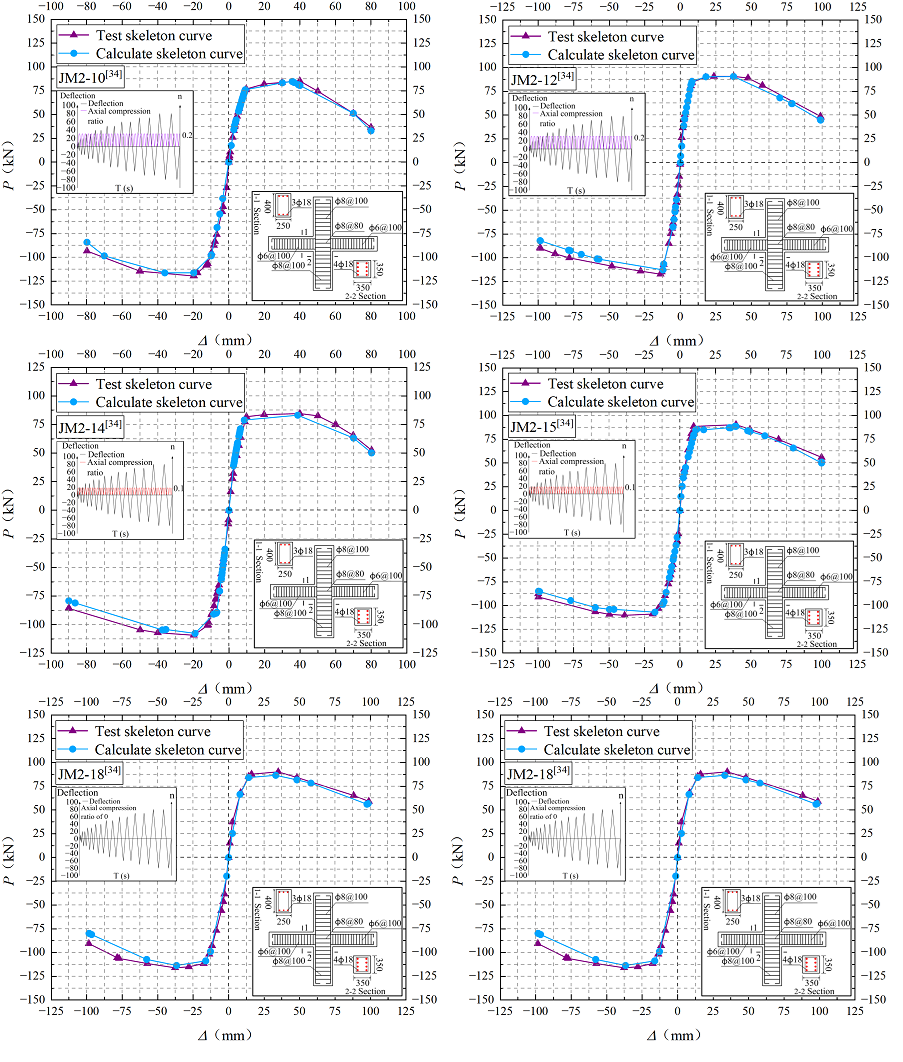
A comparison between the calculated and test skeleton curves is presented in Figure 13. The results indicate that the two curves exhibit essentially the same overall trend, with close agreement in both load and displacement at all characteristic points. The average errors corresponding to the cracking, yielding, peak, and ultimate loads are \(7.07\%\), \(5.93\%\), \(4.89\%\), and \(7.76\%\), respectively, all of which fall within an acceptable range. These results demonstrate that the proposed restoring force model can effectively capture the load–deformation behavior of beam–column joints under dynamic loading.
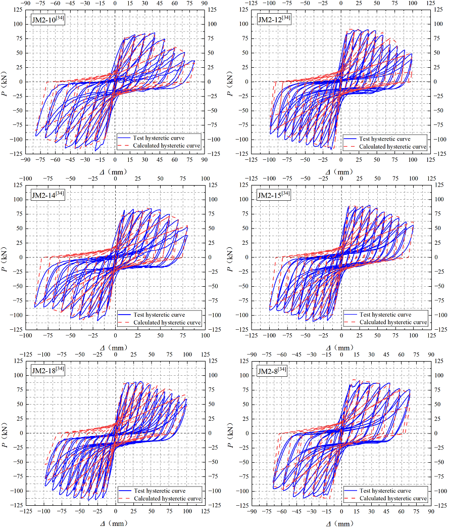
Comparisons between the calculated and test hysteretic curves are shown in Figure 14. Overall, good agreement is observed between the two sets of results. The calculated hysteretic curves accurately predict the shear capacity of the beam–column joint under dynamic loading and effectively reproduce key hysteretic characteristics, including strength degradation, stiffness degradation, and pinching behavior. Prior to reaching the peak strength, the calculated load–displacement responses closely match the test results, indicating that the restoring force model reliably captures the stiffness characteristics of the ascending branch. After the peak strength point, however, some calculated curves exhibit relatively larger deviations from the test results. This discrepancy can be attributed to the adoption of an empirical value of \(0.85P_m\), derived from quasi-static tests, as the ultimate load in the skeleton curve, whereas the actual ultimate load under dynamic loading conditions shows greater variability. Nevertheless, the overall agreement between the calculated and test hysteretic curves remains satisfactory, confirming that the proposed restoring force model is capable of effectively simulating the hysteretic behavior of beam–column joints subjected to dynamic loading.
A comparison of displacement ductility coefficients is presented in Table 3 to evaluate the capability of the restoring force model in predicting the deformation capacity of the member. To improve the reliability of the evaluation, the displacement ductility factors are determined using three different approaches based on the available data: the geometric graphic method, the equivalent elastic–plastic energy method, and the \(0.75F_u\) method. The average value obtained from these three methods is taken as the final displacement ductility coefficient. The comparison results indicate that the calculated displacement ductility coefficients show good agreement with the test values for both positive and negative loading directions. The maximum error is \(14.29\%\), while the average error is \(7.66\%\), both of which fall within an acceptable range. These results demonstrate that the proposed restoring force model is capable of effectively evaluating the deformation capacity of beam–column joints under dynamic loading.
| No. | Direction | Geometric graphic | Equivalent elastic-plastic energy | \(0.75F_u\) | Average | |||||
| Test | Calculated | Test | Calculated | Test | Calculated | Test | Calculated | \(|e|\%\) | ||
| JM2-10 [34] | Positive | 6.25 | 5.27 | 4.67 | 4.3 | 5.35 | 5.14 | 5.42 | 4.9 | 9.59% |
| Negative | 6.86 | 5.63 | 5.91 | 4.62 | 5.79 | 6 | 6.19 | 5.42 | 12.44% | |
| JM2-12 [34] | Positive | 10.7 | 10.94 | 9.41 | 8.4 | 8.8 | 8.34 | 9.64 | 9.23 | 4.25% |
| Negative | 7.83 | 7.24 | 7.43 | 7.55 | 6.93 | 7.38 | 7.4 | 7.39 | 0.14% | |
| JM2-14 [34] | Positive | 7.87 | 8.17 | 7.07 | 5.37 | 7.21 | 8.24 | 7.38 | 7.26 | 1.63% |
| Negative | 9.4 | 7.88 | 6.97 | 5.36 | 6.93 | 8.19 | 7.77 | 7.14 | 8.10% | |
| JM2-15 [34] | Positive | 8.05 | 8.15 | 7.75 | 7.23 | 7.86 | 6.53 | 7.89 | 7.3 | 7.48% |
| Negative | 9.25 | 8.32 | 7.59 | 6.31 | 7.52 | 6.98 | 8.12 | 7.2 | 11.33% | |
| JM2-18 [34] | Positive | 7.58 | 6.95 | 7.63 | 5.94 | 7.67 | 6.73 | 7.63 | 6.54 | 14.29% |
| Negative | 6.65 | 5.68 | 6.26 | 4.94 | 6.21 | 5.79 | 6.37 | 5.47 | 14.13% | |
| JM2-8 [34] | Positive | 8.3 | 8.67 | 8.08 | 7.42 | 8.43 | 7.68 | 8.27 | 7.92 | 4.23% |
| Negative | 8.71 | 7.34 | 5.38 | 5.91 | 5.43 | 5.45 | 6.51 | 6.23 | 4.30% | |
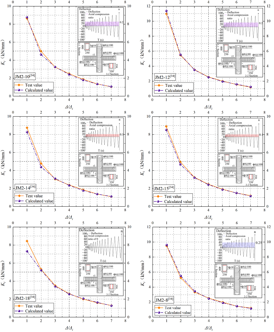
As shown in Figure 15, the stiffness degradation behavior is assessed by comparing the secant stiffness obtained from the proposed model with the test results. The comparison shows that the degradation trend of the calculated secant stiffness is in good agreement with that observed in the tests. Across different displacement amplitudes, the calculated secant stiffness values remain consistent with the test data. The maximum and average errors are \(13.27\%\) and \(4.48\%\), respectively, both within a permissible range. These results indicate that the proposed restoring force model can accurately capture the stiffness degradation characteristics of beam–column joints under cyclic loading.
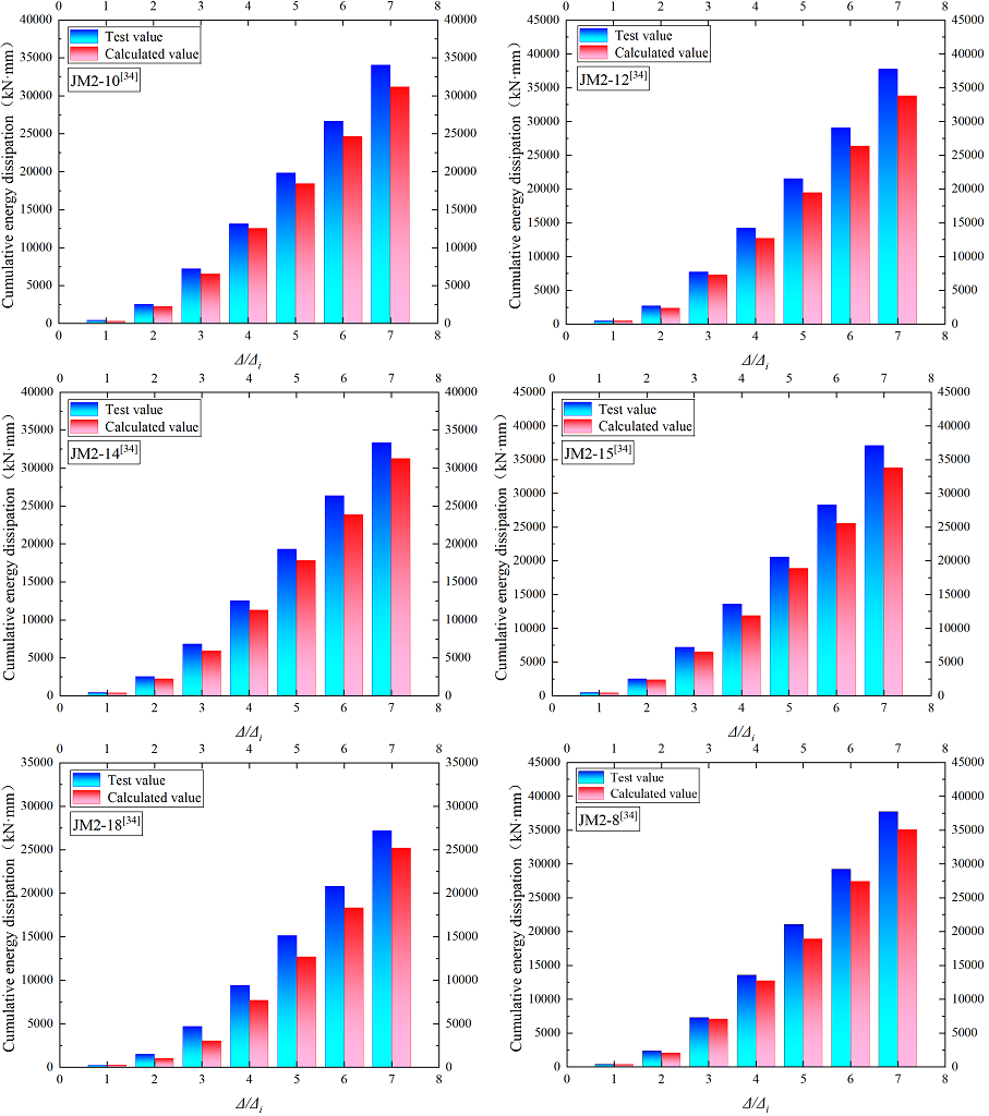
Figures 16 and 17 present comparisons of the cumulative energy dissipation and the equivalent viscous damping coefficient, respectively, to assess the model’s ability to predict the energy dissipation capacity of the member. The calculated cumulative energy dissipation at each displacement amplitude shows close agreement with the test results, although most calculated values are slightly lower than the test data. The maximum and average errors are \(13.17\%\) and \(8.80\%\), respectively, both within an acceptable range. Similarly, the equivalent viscous damping coefficient obtained from the model exhibits a high level of consistency with the test values, with maximum and average errors of \(13.83\%\) and \(8.11\%\), respectively. As shown in Figure 17, the calculated equivalent viscous damping coefficient curve closely follows the test curve during the early loading stage, while a modest deviation appears in the later stage. This deviation is mainly attributed to the fact that the hysteretic behavior in the model is derived from multiple regression analysis, which introduces inherent discrepancies in the hysteretic loop area that become more pronounced as the displacement amplitude increases. Overall, the energy dissipation parameters predicted by the proposed restoring force model show good agreement with the test results, demonstrating that the model can effectively evaluate the energy dissipation capacity of beam–column joints under dynamic loading.
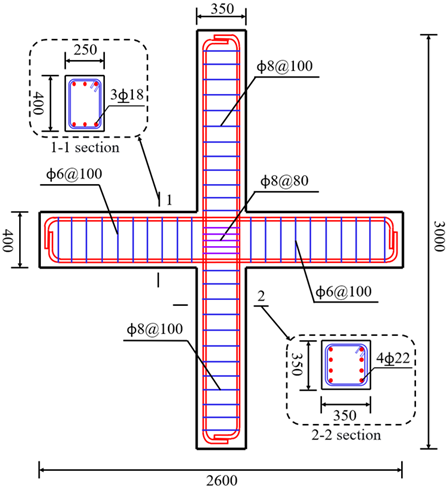
Following the design guidelines for database No. 88–101 in [34], eight beam–column joint specimens were prepared with identical cross-sectional dimensions, longitudinal reinforcement, and stirrup configurations. The concrete exhibited an average 28-day cube compressive strength of 33.21 MPa. The longitudinal reinforcement was HRB335, and the stirrups were HPB300. Detailed geometric and reinforcement parameters of the specimens are shown in Figure 18.
According to the loading protocol specified for database No. 88–101 in [34], displacement-controlled loading was applied at the beam end, while the column end was subjected to either fixed or varying axial force. The maximum axial compression ratio was set to 0.5, and the corresponding loading schemes are summarized in Table 4. Under varying axial force conditions, the axial force increased with the beam-end displacement within each loading cycle. When the beam-end displacement reached the target amplitude, the column end maintained the maximum axial force until the beam returned to its initial position, after which the axial force was reduced to zero, completing one loading cycle. This axial force variation pattern was repeated in subsequent cycles, as illustrated in Figure 19(a).
Based on the finite element modeling approach described in section 4, a numerical model of the beam–column joint was established according to the specimen design and loading protocol. The model was employed to simulate the mechanical response of the joint under complex dynamic loading conditions involving coupled variations in strain rates and axial forces.
| Load speed (mm/s) | Elastic strain rate | Plastic strain rate | Axial force loading scheme | Axial compression ratio | |
| RFM-1 | 0.4 | \(10^-4\) | \(10^-5\) | Fixed axial force | 0.5 |
| RFM-2 | 0.4 | \(10^-4\) | \(10^-5\) | Varying axial force | \(0\sim0.5\) |
| RFM-3 | 4 | \(10^-3\) | \(10^-4\) | Fixed axial force | 0.5 |
| RFM-4 | 4 | \(10^-3\) | \(10^-4\) | Varying axial force | \(0\sim0.5\) |
| RFM-5 | 40 | \(10^-2\) | \(10^-3\) | Fixed axial force | 0.5 |
| RFM-6 | 40 | \(10^-2\) | \(10^-3\) | Varying axial force | \(0\sim0.5\) |
| RFM-7 | 400 | \(10^-1\) | \(10^-2\) | Fixed axial force | 0.5 |
| RFM-8 | 400 | \(10^-1\) | \(10^-2\) | Varying axial force | \(0\sim0.5\) |
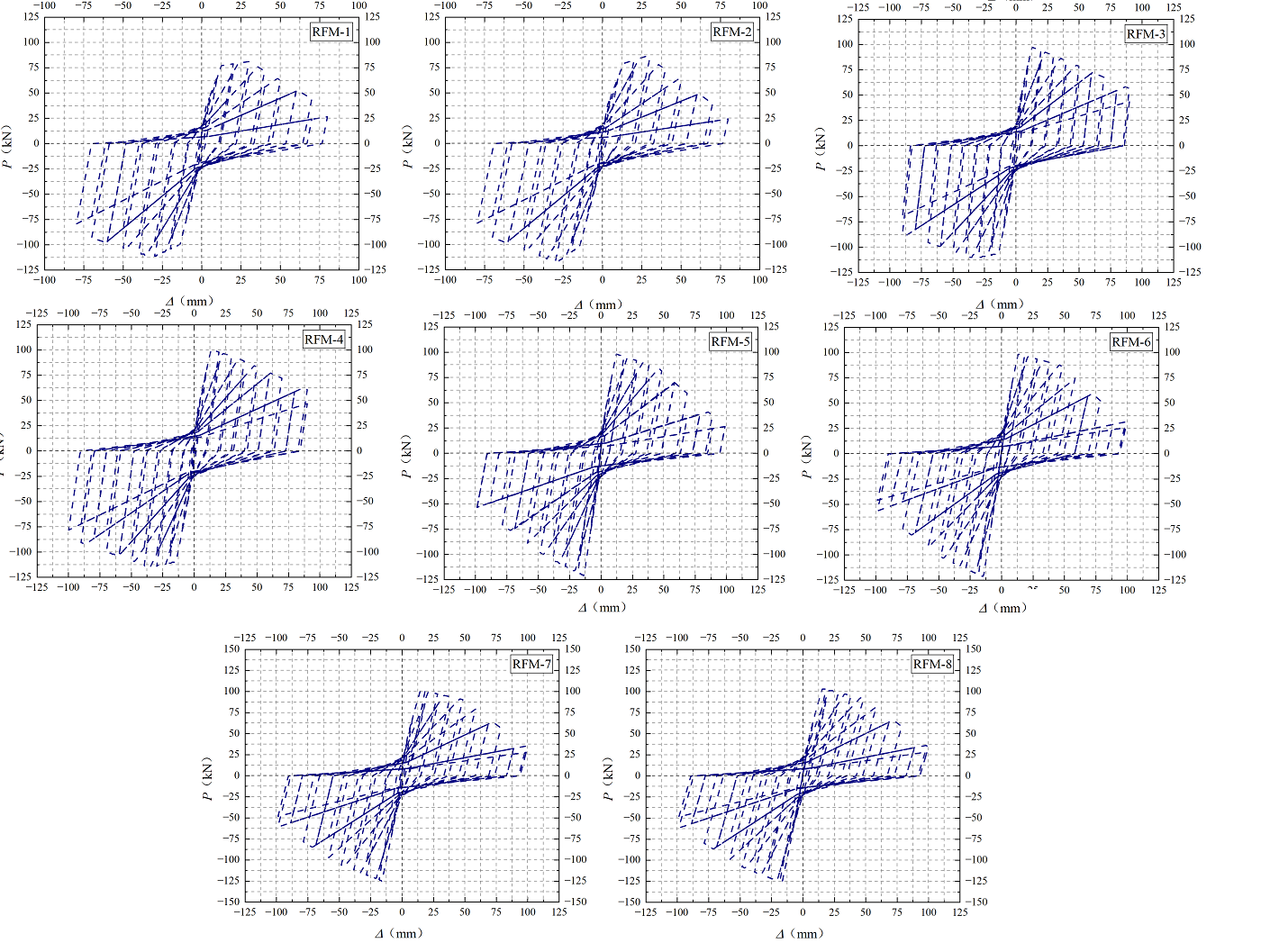
The simulated hysteretic curves are presented in Figure 20. The results indicate that the overall shapes of the hysteretic curves obtained under varying axial force are very similar to those under fixed axial force, demonstrating good consistency between the two loading conditions. Under coupled varying strain rates and axial forces, the evolution of the hysteretic response of the beam–column joint can be summarized as follows. (1) In the initial loading stage, the hysteretic curve exhibits a nearly linear response, with the unloading stiffness close to the initial elastic stiffness. At this stage, the influence of varying strain rates and axial forces is negligible. (2) With increasing load, pinching behavior begins to appear in the hysteretic curve, and residual deformation gradually becomes evident. (3) As loading continues, the residual deformation of the hysteretic loops increases, accompanied by a more pronounced degradation of stiffness. (4) When the member reaches the peak load, two hysteretic loops are observed at the same displacement amplitude. The peak load of the second loop is lower than that of the first, and a descending branch emerges, indicating significant strength degradation. (5) Beyond the peak load, both strength and stiffness degradation become more severe, and the pinching effect is further intensified.
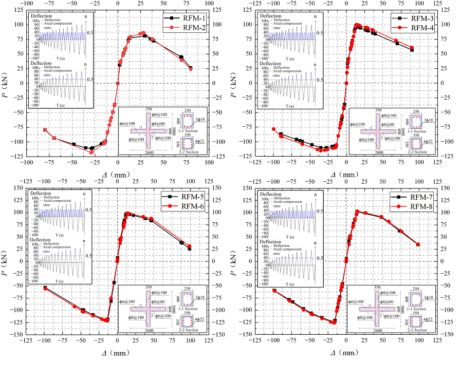
As shown in Figure 21, the skeleton curves are extracted from the hysteretic curves of the beam–column joint using the envelope method. Under varying axial force, the average positive and negative ultimate carrying capacities are slightly higher than those under the fixed axial force, with a maximum increase of \(4.35\%\). Although the load in the descending branch exhibits merely a slight increase, the overall shape of the skeleton curves remains consistent under both conditions. Furthermore, both the yield and ultimate carrying capacities of the beam–column joint are notably enhanced at higher strain rates. The improvement in ultimate carrying capacity is more substantial than that in yield carrying capacity, reaching a maximum of approximately \(25.77\%\). Concurrently, the descending branch becomes steeper, indicating that stiffness degradation intensifies with increasing strain rate.
The displacement ductility coefficient \(\mu_\Delta\) is employed to analyze the deformation capacity of beam–column joints under varying strain rates and axial forces. The formula is expressed as: \[\mu_\Delta=\frac{\Delta_u}{\Delta_y}. \label{eq50} \tag{50}\]
The data are processed in accordance with the method in Section 4.3, and the results are shown in Table 5. At lower strain rate (\(\dot{\varepsilon}\le10^{-4}\,\mathrm{s^{-1}}\)), the displacement ductility coefficient under varying axial force decreases by up to \(22.3\%\) compared with that under fixed axial force. However, at higher strain rate (\(\dot{\varepsilon}>10^{-4}\,\mathrm{s^{-1}}\)), the displacement ductility coefficient under varying axial force shows only minor variation, with a maximum reduction of \(6.58\%\). This indicates that varying axial force generally leads to a reduction in the displacement ductility coefficient. However, the rate of degradation decreases rapidly with increasing strain rate, causing the displacement ductility coefficient under varying axial force to gradually approach that under fixed axial force. Therefore, the influence of varying axial force on member ductility becomes relatively minor at higher strain rates (\(\dot{\varepsilon}>10^{-4}\,\mathrm{s^{-1}}\)).
In addition, increasing strain rate results in a pronounced reduction in the displacement ductility coefficient of the beam–column joint, with a maximum decrease of \(26.21\%\). This finding confirms that the deformation capacity of the beam–column joint deteriorates as the strain rate increases.
| No. | Direction | Geometric graphic | Equivalent elastic–plastic energy | \(0.75F_u\) | Average | Grand mean |
| RFM-1 | Positive | 4.67 | 4.02 | 3.80 | 4.16 | 4.35 |
| Negative | 4.62 | 4.42 | 4.57 | 4.54 | ||
| RFM-2 | Positive | 3.55 | 3.15 | 3.06 | 3.25 | 3.38 |
| Negative | 3.57 | 3.40 | 3.54 | 3.50 | ||
| RFM-3 | Positive | 5.12 | 4.46 | 3.89 | 4.49 | 5.15 |
| Negative | 5.90 | 5.90 | 5.63 | 5.81 | ||
| RFM-4 | Positive | 5.71 | 4.51 | 4.01 | 4.74 | 5.01 |
| Negative | 5.27 | 5.22 | 5.22 | 5.24 | ||
| RFM-5 | Positive | 5.67 | 4.58 | 4.26 | 4.84 | 4.02 |
| Negative | 3.14 | 3.23 | 3.20 | 3.19 | ||
| RFM-6 | Positive | 4.85 | 4.37 | 4.18 | 4.47 | 3.88 |
| Negative | 3.25 | 3.29 | 3.29 | 3.28 | ||
| RFM-7 | Positive | 5.29 | 4.28 | 3.97 | 4.51 | 3.80 |
| Negative | 3.02 | 3.15 | 3.09 | 3.09 | ||
| RFM-8 | Positive | 4.45 | 3.99 | 3.81 | 4.08 | 3.55 |
| Negative | 2.97 | 3.05 | 3.03 | 3.02 |
Stiffness degradation, which reflects the accumulation of damage under cyclic loading, is evaluated for the beam–column joint under varying strain rates and axial forces using the secant stiffness. The secant stiffness is defined as: \[K_i=\frac{\left|F_i^{+}\right|+\left|F_i^{-}\right|} {\left|\Delta_i^{+}\right|+\left|\Delta_i^{-}\right|}, \label{eq51} \tag{51}\] where \(F_i^{+}\) and \(F_i^{-}\) are the positive and negative peak loads at the \(i\)-th displacement amplitude, while \(\Delta_i^{+}\) and \(\Delta_i^{-}\) are the corresponding positive and negative peak displacements.
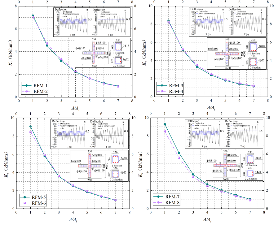
The secant stiffness curves are shown in Figure 22. At lower strain rates (\(\dot{\varepsilon}\le10^{-3}\,\mathrm{s^{-1}}\)), the secant stiffness curves under varying and fixed axial force are nearly identical. At higher strain rates (\(\dot{\varepsilon}>10^{-3}\,\mathrm{s^{-1}}\)) and lower displacement amplitude \((\Delta/\Delta_u<3)\), the secant stiffness under varying axial force is slightly higher than under fixed axial force, with a maximum increase of \(8.28\%\). As the displacement amplitude increases, the secant stiffness gradually converges to that obtained under fixed axial force, indicating that the influence of varying axial force on stiffness degradation is limited. In contrast, the effect of strain rate on stiffness is more pronounced. With increasing strain rate, the secant stiffness of the beam–column joint increases over the entire range of displacement amplitudes, with a maximum increase of \(22.9\%\). This result indicates that higher strain rates generally enhance the stiffness of the member. However, at larger displacement amplitudes, stiffness degradation becomes increasingly significant as the strain rate rises.
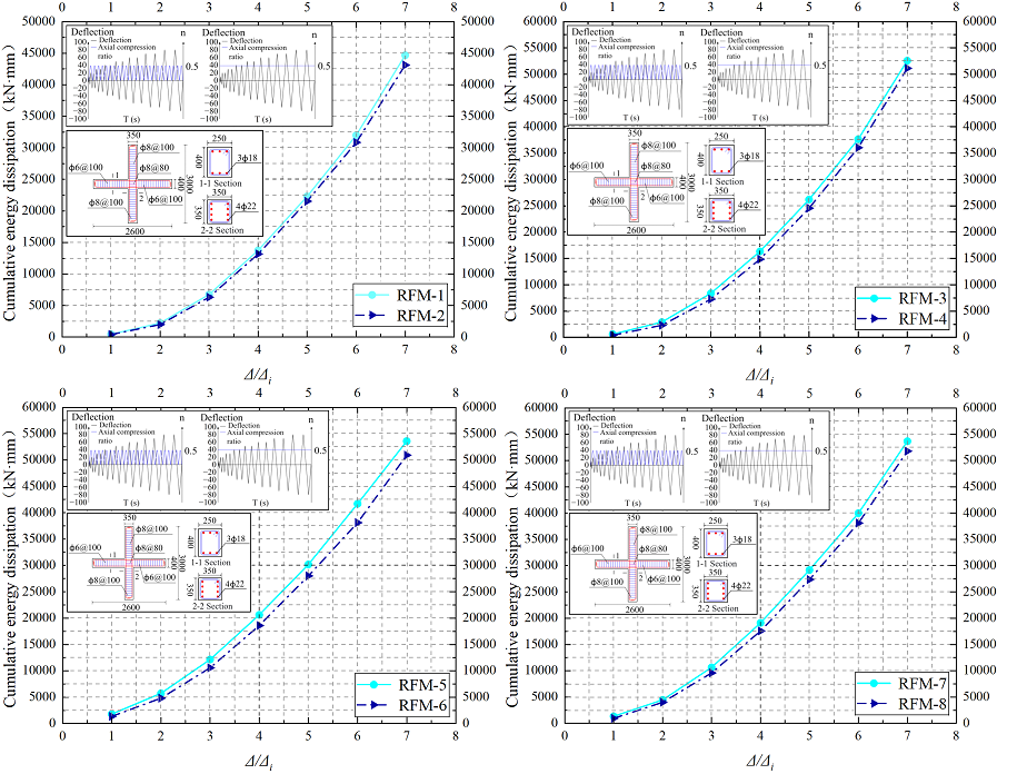
Cumulative energy dissipation and the equivalent viscous damping coefficient are commonly used to evaluate the energy dissipation capacity of beam–column joints. Cumulative energy dissipation is obtained by summing the areas enclosed by the hysteretic loops and reflects the energy dissipation capacity of the member under cyclic loading, as shown in Figure 23. Under varying axial force, the cumulative energy dissipation of the beam–column joint is slightly lower than that under fixed axial force across different displacement amplitudes, with a maximum reduction not exceeding \(11.09\%\). The overall shapes of the curves corresponding to the two loading conditions remain highly similar. Furthermore, when the strain rate is below \(10^{-3}\,\mathrm{s^{-1}}\), the cumulative energy dissipation at higher strain rates exceeds that at lower strain rates, with a maximum increase of \(33.34\%\). When the strain rate exceeds \(10^{-3}\,\mathrm{s^{-1}}\), the opposite trend emerges. This indicates that the cumulative energy dissipation increases with the strain rate within a specific range (\(\dot{\varepsilon}=10^{-5}\,\mathrm{s^{-1}}\sim10^{-3}\,\mathrm{s^{-1}}\)).
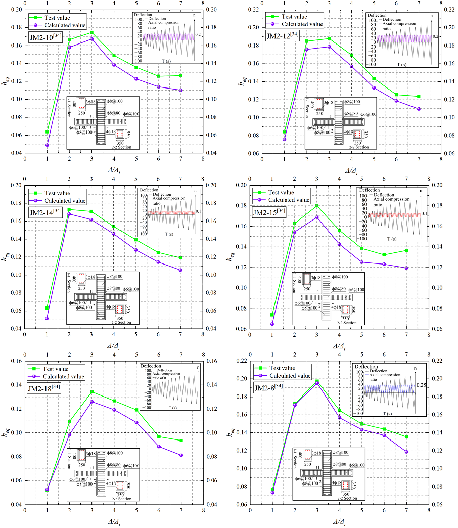
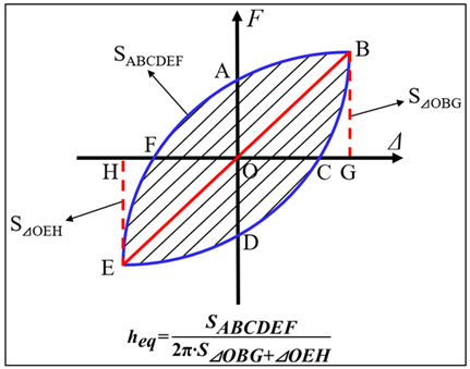
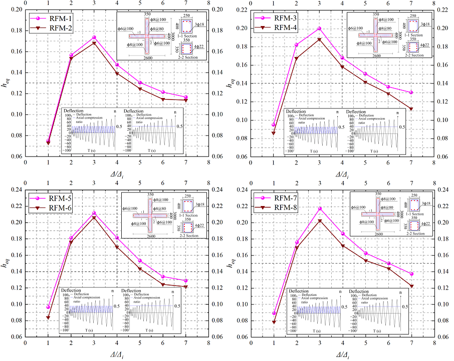
The equivalent viscous damping coefficient \(h_{eq}\) quantifies the energy dissipation efficiency associated with the shape of the hysteretic loop. To comprehensively evaluate the energy dissipation capacity of beam–column joints under varying strain rates and axial forces, \(h_{eq}\) is combined with the cumulative energy dissipation. The relevant formulations and corresponding curves are shown in Figures 24 and 25, respectively. When subjected to varying axial force, \(h_{eq}\) exhibits a slight decrease across all displacement amplitudes compared to the fixed axial force, with reduction ranging from \(1.91\%\) to \(12.5\%\). Meanwhile, the curves corresponding to the two axial force conditions display a high degree of similarity. Combined with the cumulative energy dissipation results discussed above, this indicates that varying axial force has a limited influence on the overall energy dissipation capacity. As the strain rate increases, \(h_{eq}\) rises at all displacement amplitudes, with a maximum increase of \(22.73\%\). The simultaneous enhancement of both cumulative energy dissipation and equivalent viscous damping coefficient demonstrates that the beam–column joint dissipates more energy at higher strain rates.
This study proposes an asymmetric rate-dependent restoring force model for beam-column joint subjected to varying strain rates and axial forces. The model is used to investigate the dynamic performance of beam-column joint. The main conclusions are as follows:
(1) Based on the characteristics of the complete force-deformation behavior of beam-column joint, a quadrilinear skeleton curve is developed, which is defined by four key points corresponding to cracking, yielding, peak strength, and ultimate strength. By combining parametric analysis with the mean value theorem, explicit expressions for these characteristic points are obtained via strip integration, accounting for the effects of variable strain rates and axial forces. The resulting formulations accurately predict the load–displacement response of beam-column joint under complex dynamic loading characterized by coupled variations in strain rate and axial force.
(2) Based on the proposed skeleton curve and hysteretic rules, an asymmetric rate-dependent restoring force model for beam-column joint under varying strain rates and axial forces is formulated. This model is implemented in a finite element framework to simulate the joint’s dynamic performance. The results show good agreement with test data, confirming the model’s effectiveness in analyzing the dynamic performance of the beam-column joint under complex dynamic loading.
(3) At higher strain rate, both the yield and ultimate carrying capacities of the beam-column joint increase, with the ultimate carrying capacity exhibiting a greater improvement. Additionally, the increased strain rate enhances both the stiffness and energy dissipation capacity. However, these improvements are accompanied by a reduction in ductility.
(4) Under varying axial force, the hysteretic and skeleton curves of the beam-column joint closely resemble those obtained under fixed axial force. Although a slight reduction in ductility is observed, the stiffness and energy dissipation capacity remain comparable between the two loading conditions. Given these minor differences, the influence of varying axial force on dynamic performance is negligible compared to that of varying strain rate. Therefore, the distinction between varying and fixed axial force loading is practically insignificant.
This work was supported by National Natural Science Foundation of China (Grant No. 52008385), Natural Science Foundation of Shandong Province (Grant No. ZR2018BEE041), Research Subject Supported by Enterprise and Institution (20250301). The authors would like to express their gratitude for the support.
The authors declare no conflict of interest.